Explore materials in Reality Composer Pro
Explore materials in Reality Composer Pro
The next step Apple suggest is to learn about the working with USD(Universal Scene Description) files using Reality Composer Pro, here is the next step after Meet Reality Composer Pro
“Learn how Reality Composer Pro can help you alter the appearance of your 3D objects using RealityKit materials. We’ll introduce you to MaterialX and physically-based (PBR) shaders, show you how to design dynamic materials using the shader graph editor, and explore adding custom inputs to a material so that you can control it in your visionOS app. To get the most out of this session, we recommend first watching “Meet Reality Composer Pro.” Once you’re ready to learn how you can incorporate your models and materials into an Xcode project, check out “Work with Reality Composer Pro content in Xcode.” -Apple
Materials in xrOS
- What are materials?
- Materials are what define the appearance of your object in 3D scenes. Materials can be simple, just a single color, or they can use images.You might apply a wood texture to the model of a chair or map an image of bricks to a wall. Materials can also be quite sophisticated. They might use animation to look like rippling water or change appearance based on viewing angle. Think of the iridescent sparkle of mother of pearl. Materials can even modify the geometry of the objects they are applied to.
- Physical Based Rendering
- Materials in visionOS use Physically Based Rendering (PBR) to represent physical properties of real world objects, for example, how metallic or how rough an object looks.
- Let’s look at some examples of physically based materials in action.
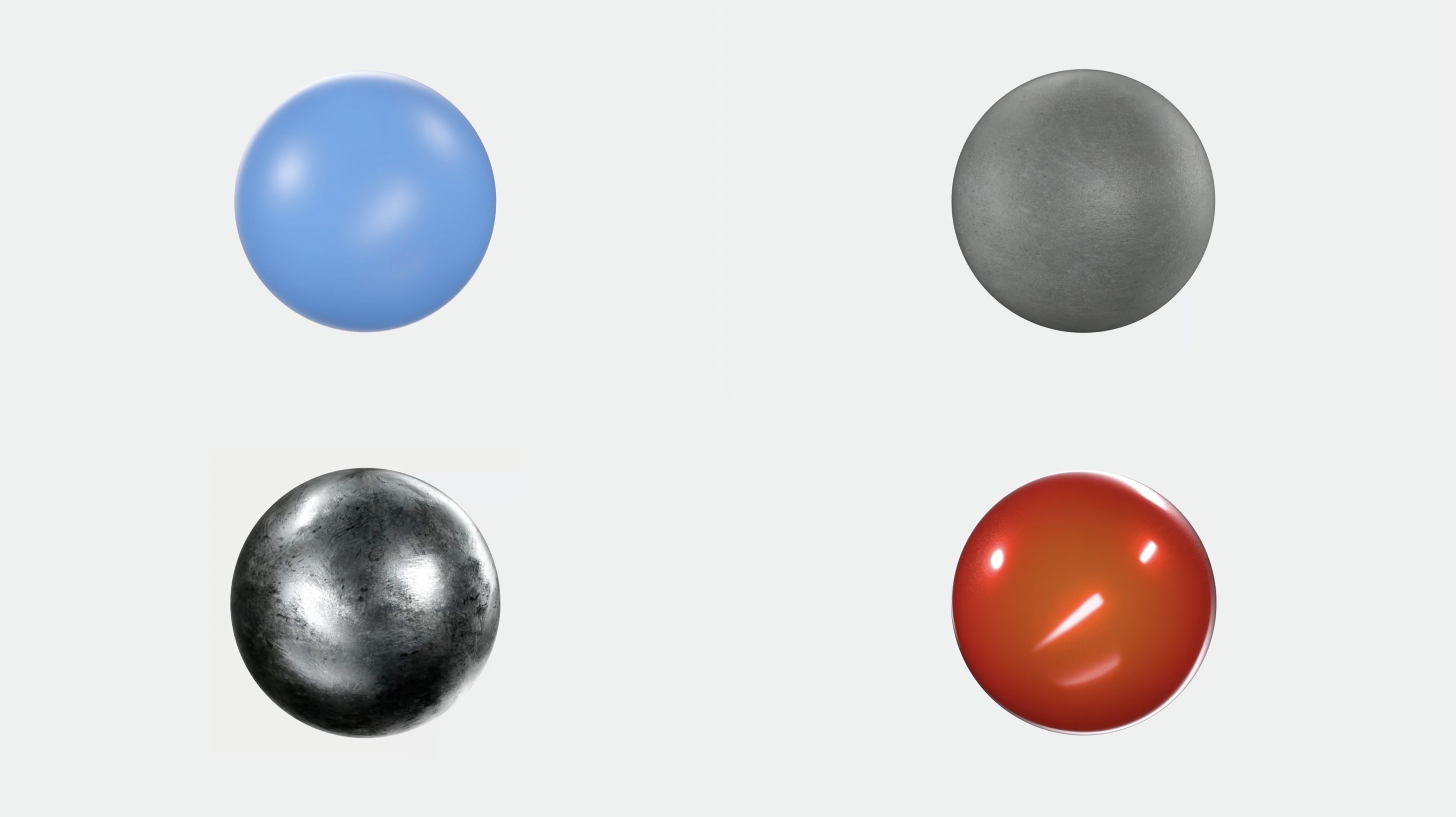
- Materials consist of one or more shaders. These are programs that do the actual work of computing the appearance of their material.
- With RealityKit 2 for iOS and iPadOS, we introduced CustomMaterial. Shaders in CustomMaterial are hand coded in Metal.

- Surface shaders operate on the PBR attributes of models. Geometry modifiers operate on the geometry of your objects.
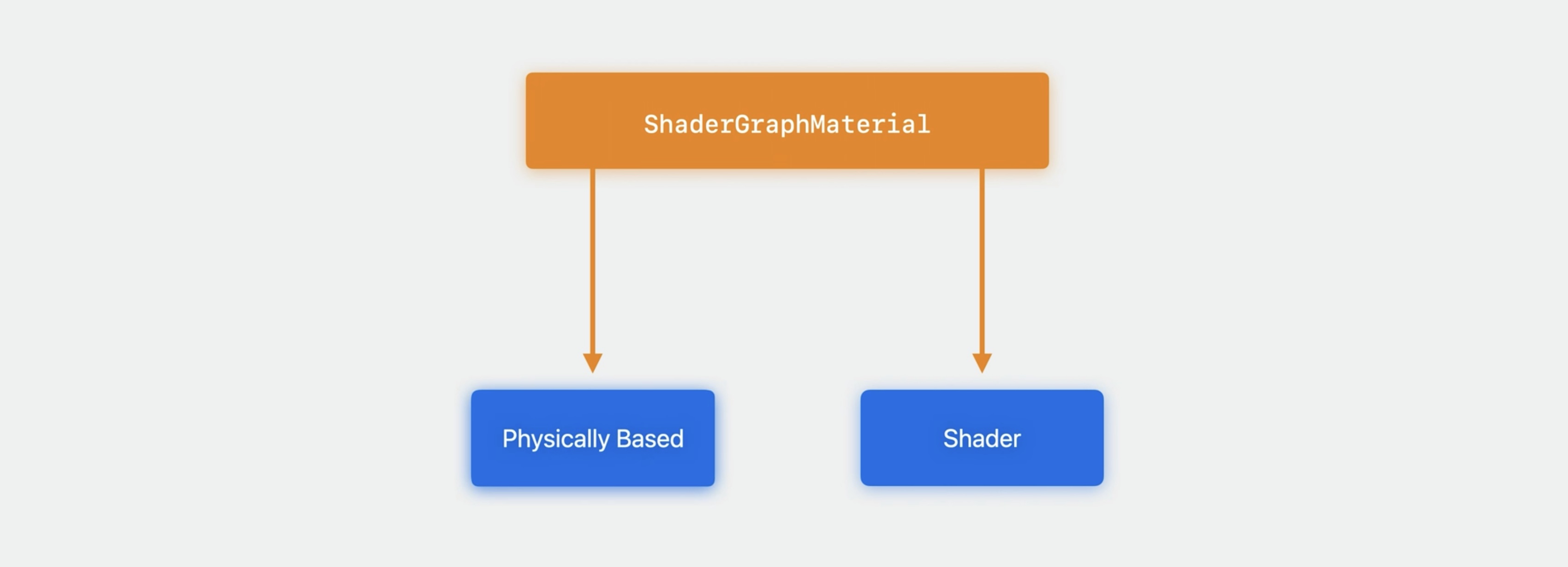
- ShaderGraphMaterial a new type of material is introduced: ShaderGraphMaterial.

-
This is the exclusive way of creating custom materials for visionOS.Based on the open standard MaterialX. Shader graph uses networks or node blocks.
- Supports 2 main types of shaders: Physically Based and Custom.
-
- Physically based shader is intended for simpler use cases (e.g. constant, non-changing values)
- Custom is intended for precise and custom control over 3D objects (e.g. animation, geometry modifiers, special effects, etc,
- Custom shaders can incorporate animation, adjust your object’s geometry, and create special effects on the surface of your object, like a sparkly paint look.
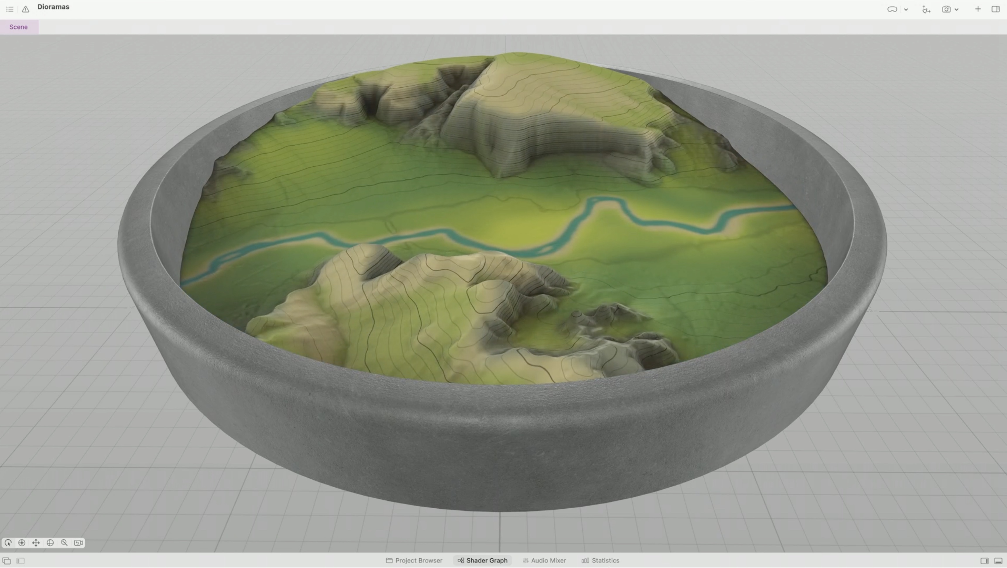
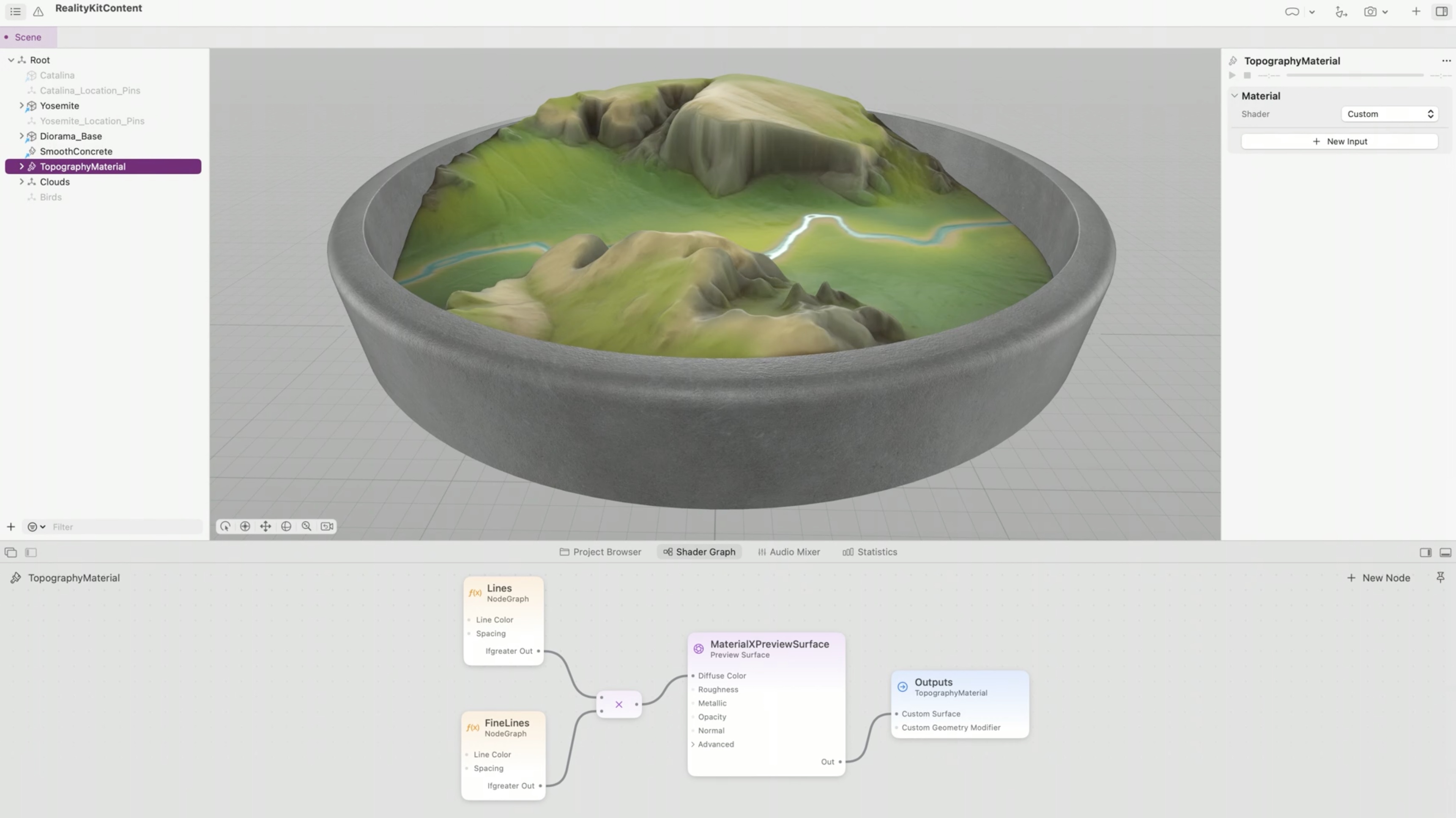
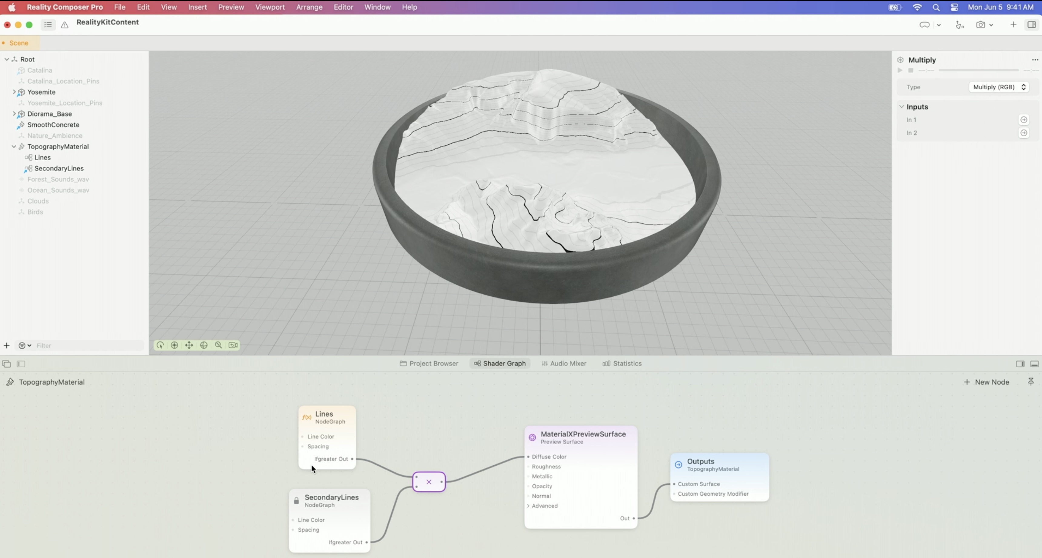
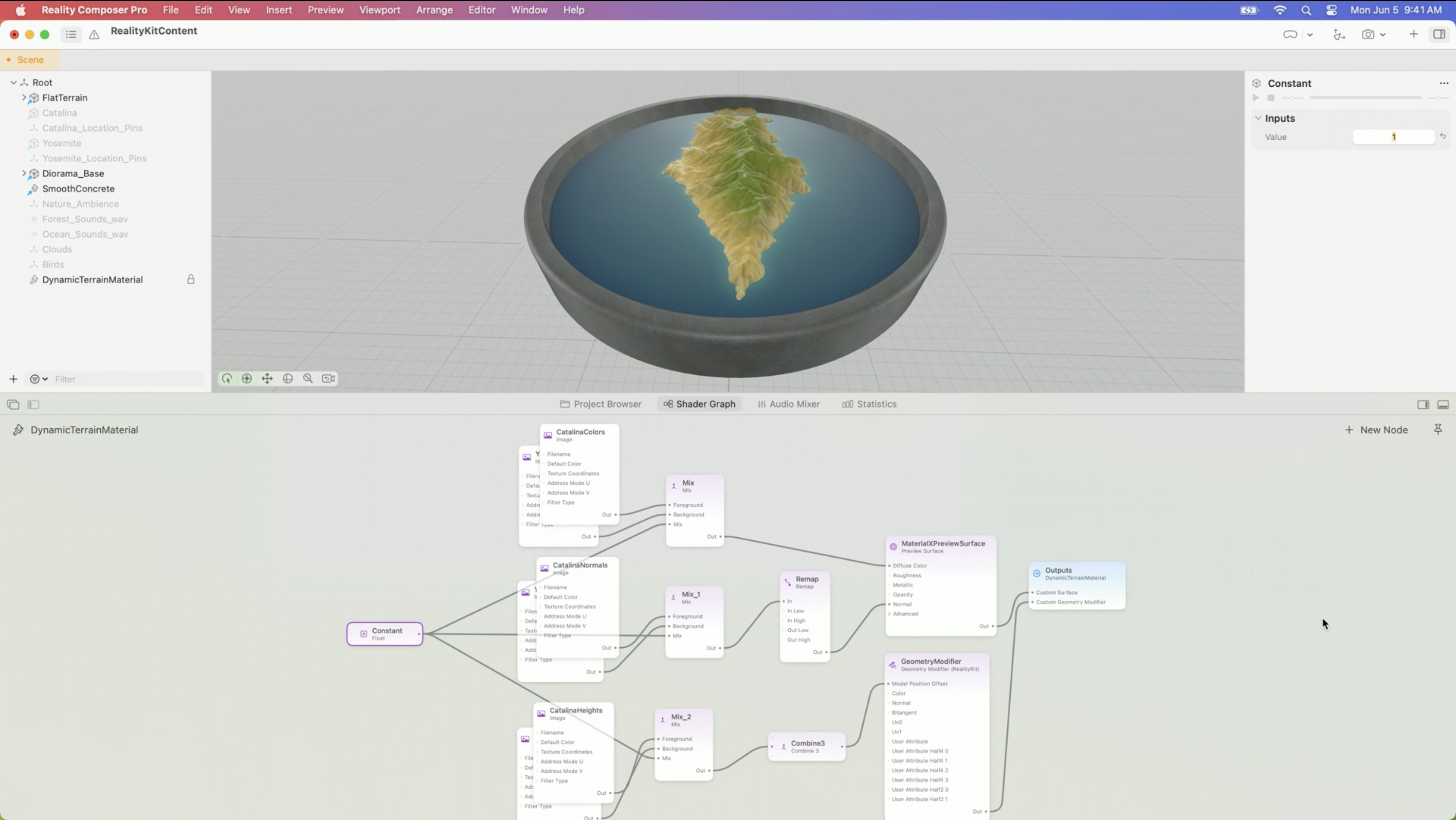
- You can build ShaderGraphMaterials using the Shader Graph editor right inside Reality Composer Pro. Take a look at the Shader Graph nodes below that instantaneously define the look of the terrain in the viewport.

Material Editing
- Materials in xrOS can be created using Reality Composer Pro
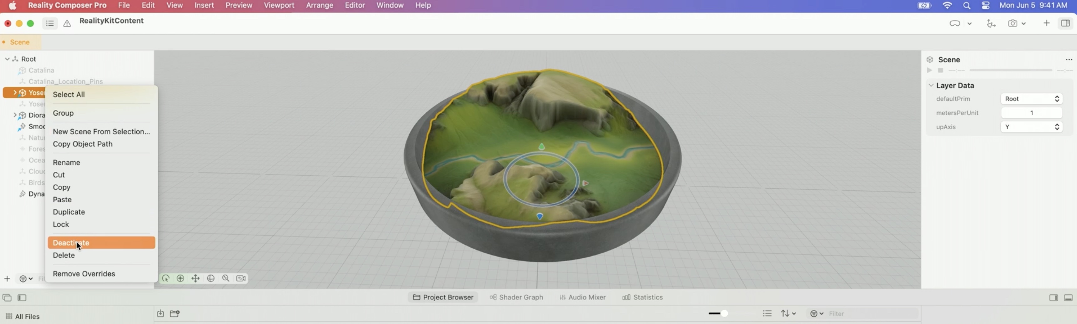
- We’ll use the Yosemite Valley model that was shown in that session and apply a topographical map appearance to it. I’ll explain the math behind our material, then we’ll go into Reality Composer Pro’s shader editor and build it. To save on time, I hid all the objects we don’t need for this session using the Deactivate command. Starts at 4:31
- Let’s add a topography feature. We’ll add a material showing the topography of our model by displaying contour lines along the slope of the terrain. It’ll look similar to the topographical map that you might have come across when planning a hike.
-
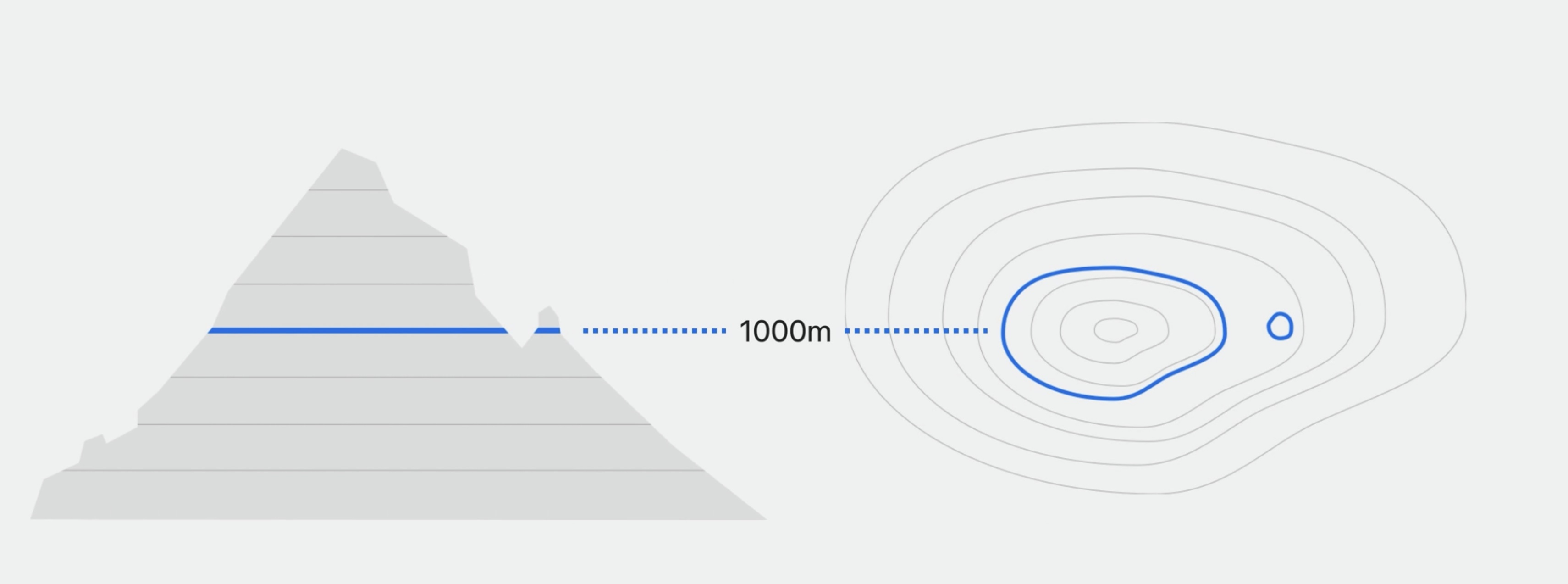
- Let’s create a custom material containing a shader that will draw contour lines on our terrain. We want to draw lines on our terrain through all the areas that have the same elevation, like in this diagram. This blue line, for example, shows all points on the terrain at 1000 meters of elevation. Seen from above, it will look something like the diagram on the right.
- Add a material by clicking the + icon inside the Project Browser. Under Materials, notice our two shader types: Physically Based and Custom. Choose Custom.
-
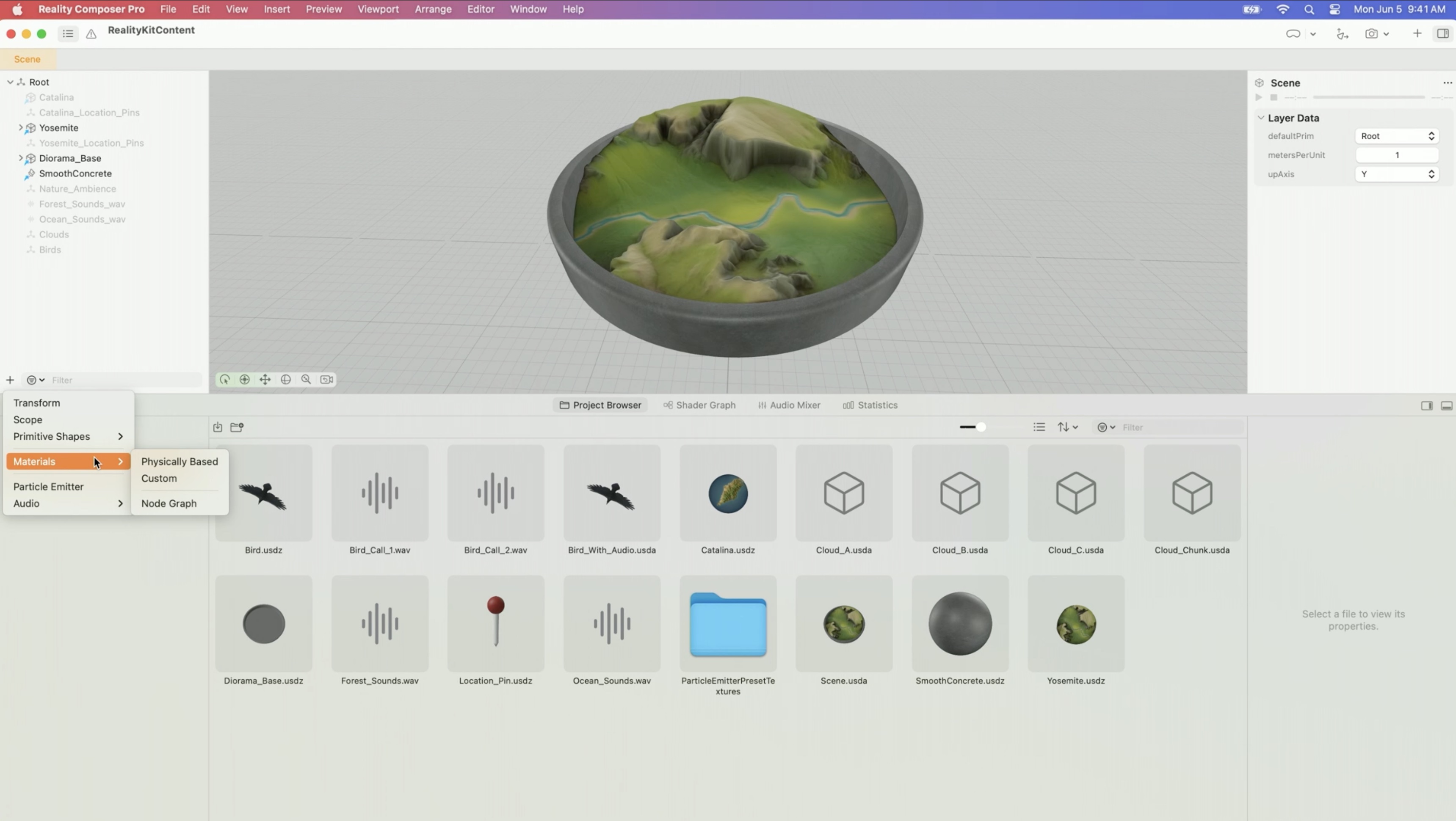
- This reveals the Shader Graph of our editor.
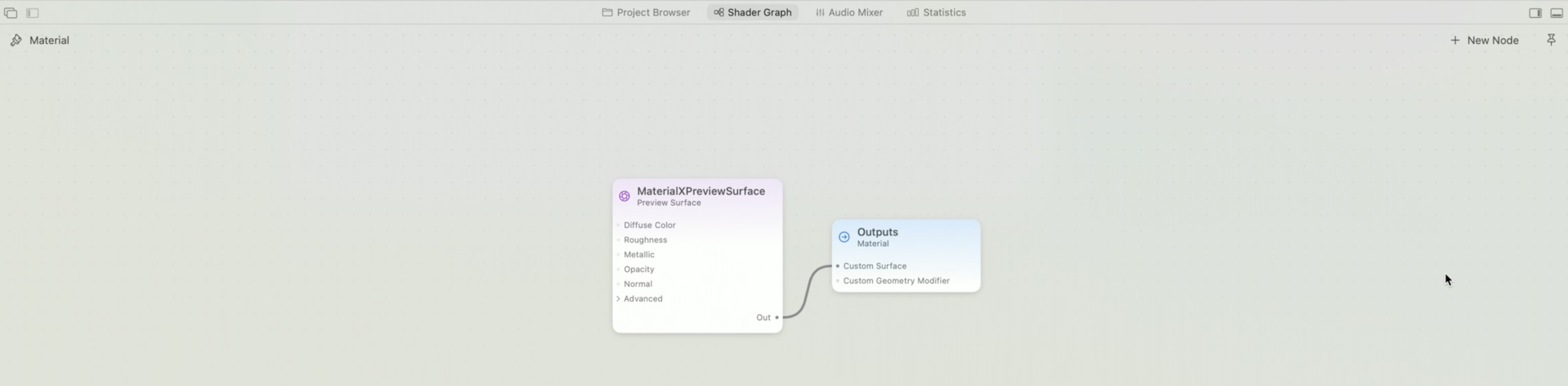
- New custom shaders start with two nodes, the surface node in purple and the outputs node in blue. Your material’s active surface is the one connected to the custom surface input of the outputs node. The inputs on the surface are how you set your shader’s physically based, or PBR, parameters. Base color, for example.
- Let’s give the material a descriptive name. TopographyMaterial sounds good. An important step is to assign our new material to our Yosemite Valley model. Select it in the project hierarchy. In the inspector, under Material Bindings, choose TopographyMaterial from the Binding menu. Important! make sure you assign your new material to your model in the hierarchy. You do this by selecting your custom material from the model’s Material Binding dropdown in the inspector 5:48.
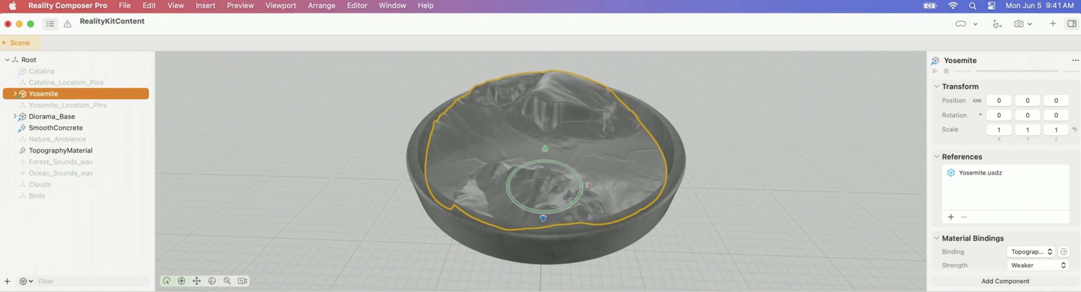
- Notice the model changes from color to a simple gray. Our material is working, but it doesn’t do anything interesting yet. Let’s fix that. Select TopographyMaterial from the hierarchy to return to the Shader Graph editor. We’ll connect some nodes to our surface inputs to draw stripes on our model in the right places.
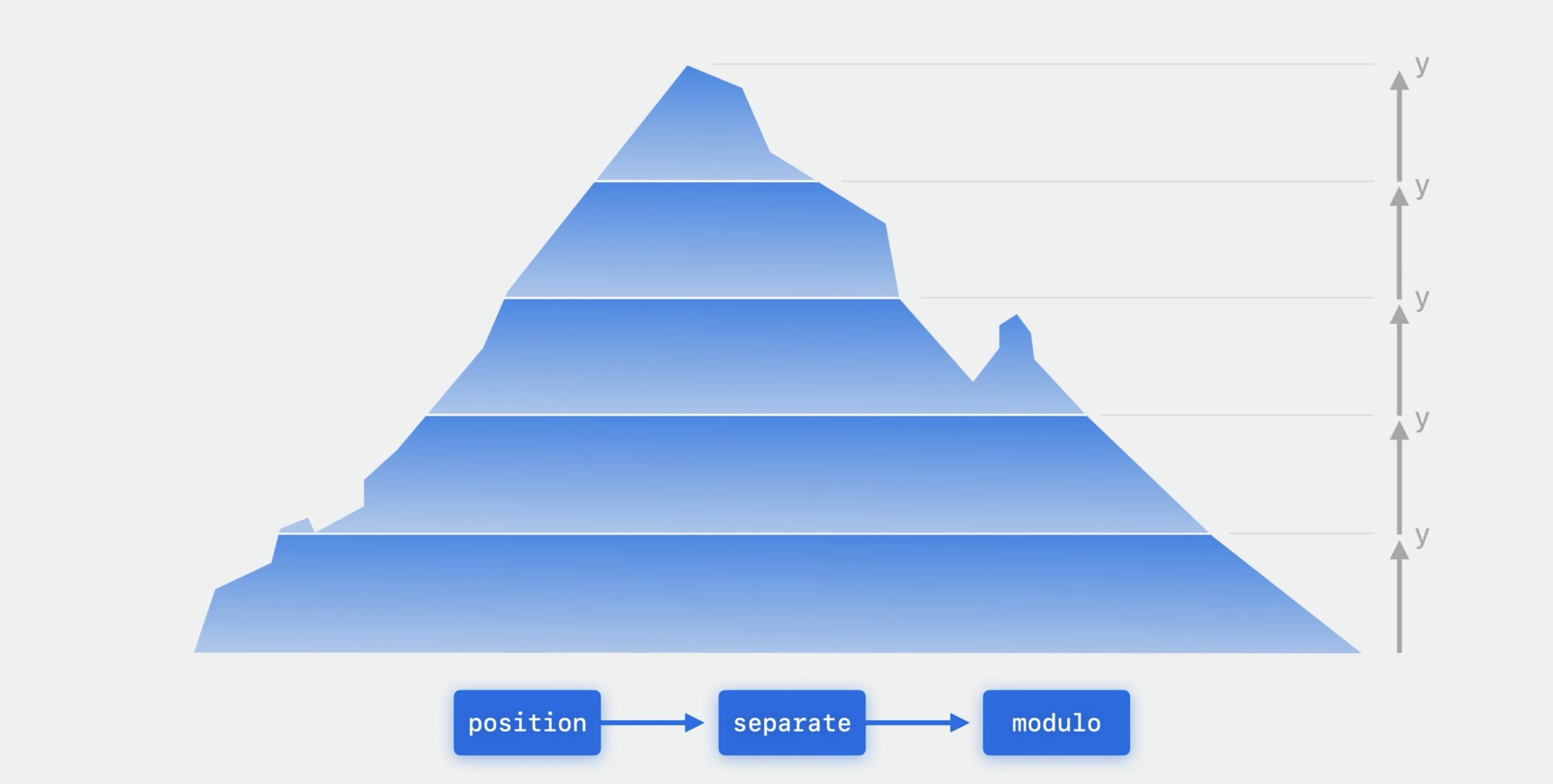
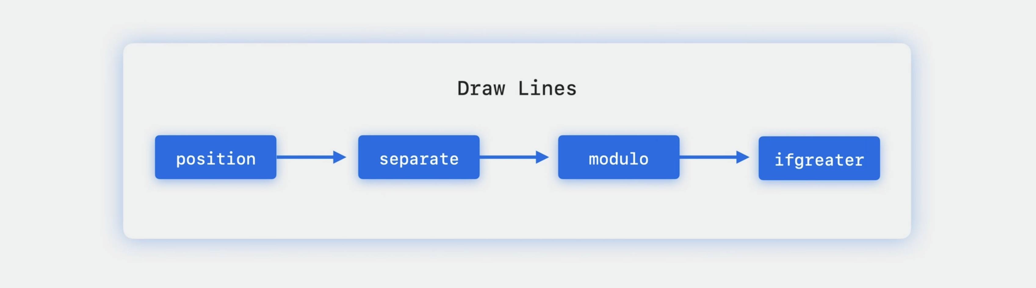
- I’ll illustrate how our material will work with this example terrain. We need our material to decide where to draw topographical lines based on its location on our model. So first we’ll add a position node to our material. This node returns our rendering position in 3D space. We’re only interested in the height of position, so we’ll also add a node called separate to extract just the position’s Y-coordinate. Separate returns the Y-coordinate position, which increases with terrain height.
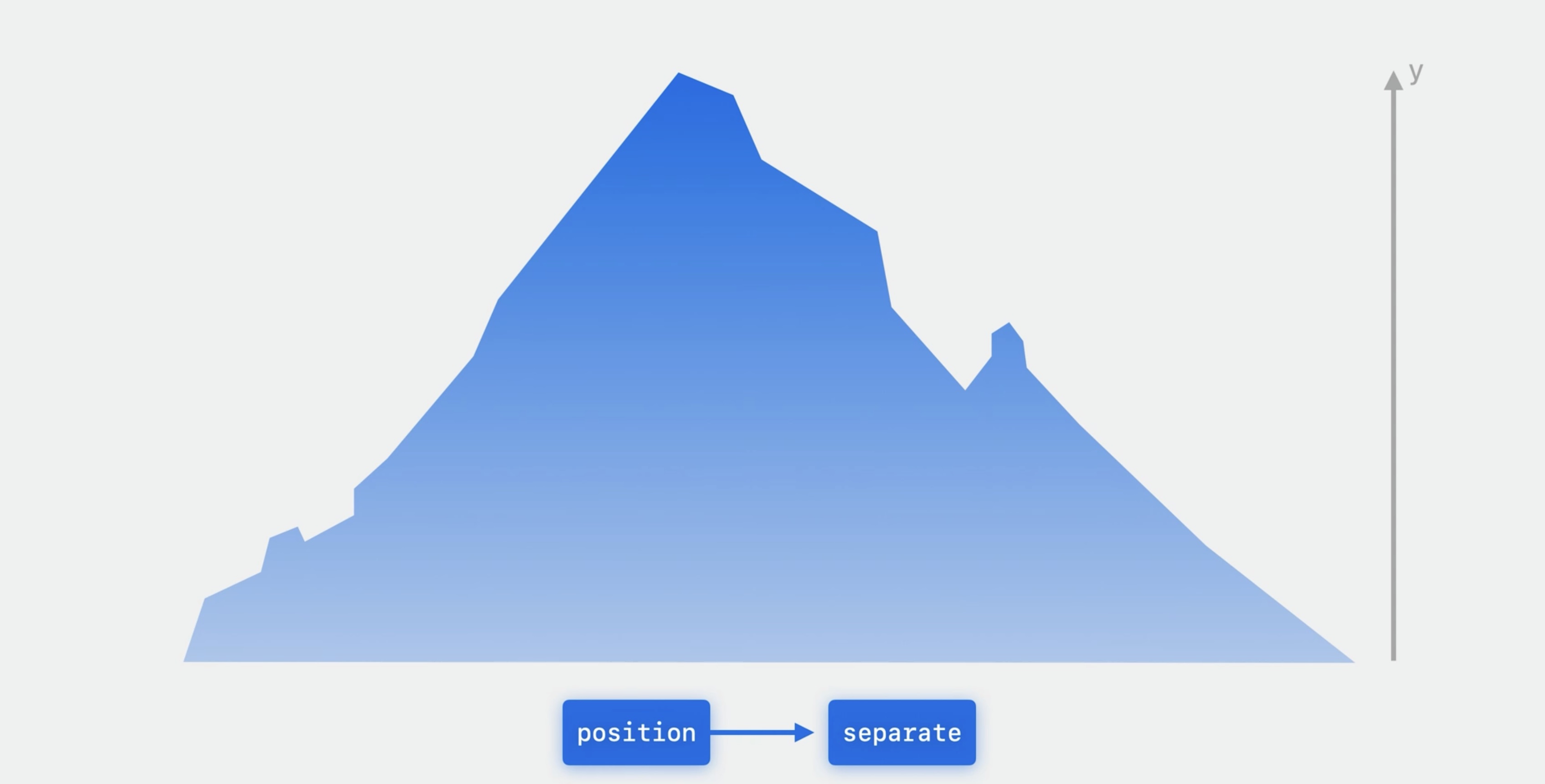
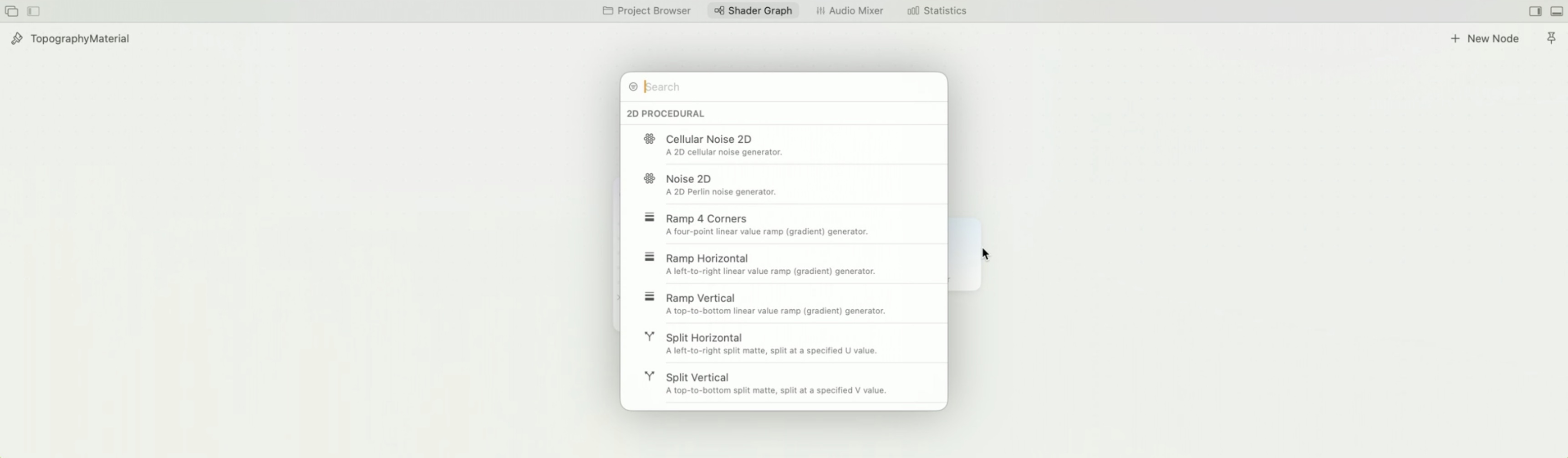
- Let’s add these first two nodes to our material in Reality Composer Pro. Double-click on the background of the editor to add nodes. This brings up the New Node picker. You can browse through the list of all the available nodes, or search for nodes by name or keyword. Let’s type “position” and select the Position node from the list to insert it into our shader. Position outputs the location in 3D space where the material is being rendered.
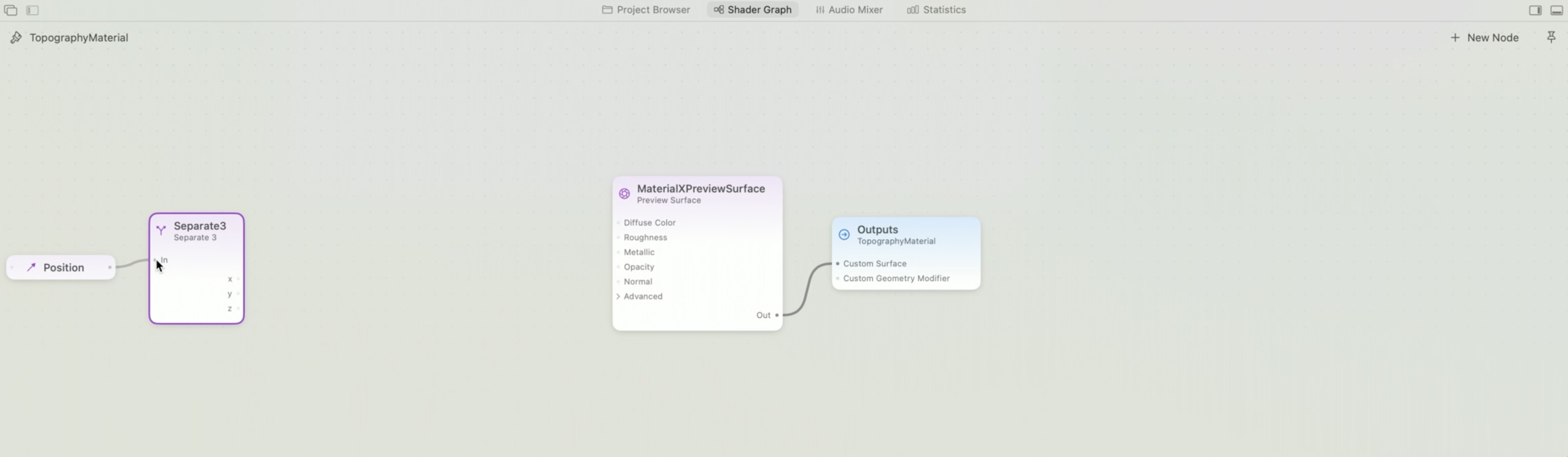
- Our material varies with height, so let’s add a separate node to extract the Y component of position. Double-click the background to bring up the New Node picker again and add a Separate 3 node. To make connections in the editor, just click and drag from node outputs to node inputs like this.
- These two nodes combined give us the height of the terrain. Next, we’ll take the output of the separate node and pass it to a modulo node. Modulo gives the remainder of dividing two values. We’ll use modulo to divide height by our desired topographical line spacing. The result looks like this. You can see height has been divided into bands. The height values inside each range start at 0 and increase to that range’s height. This will be important for our next step.
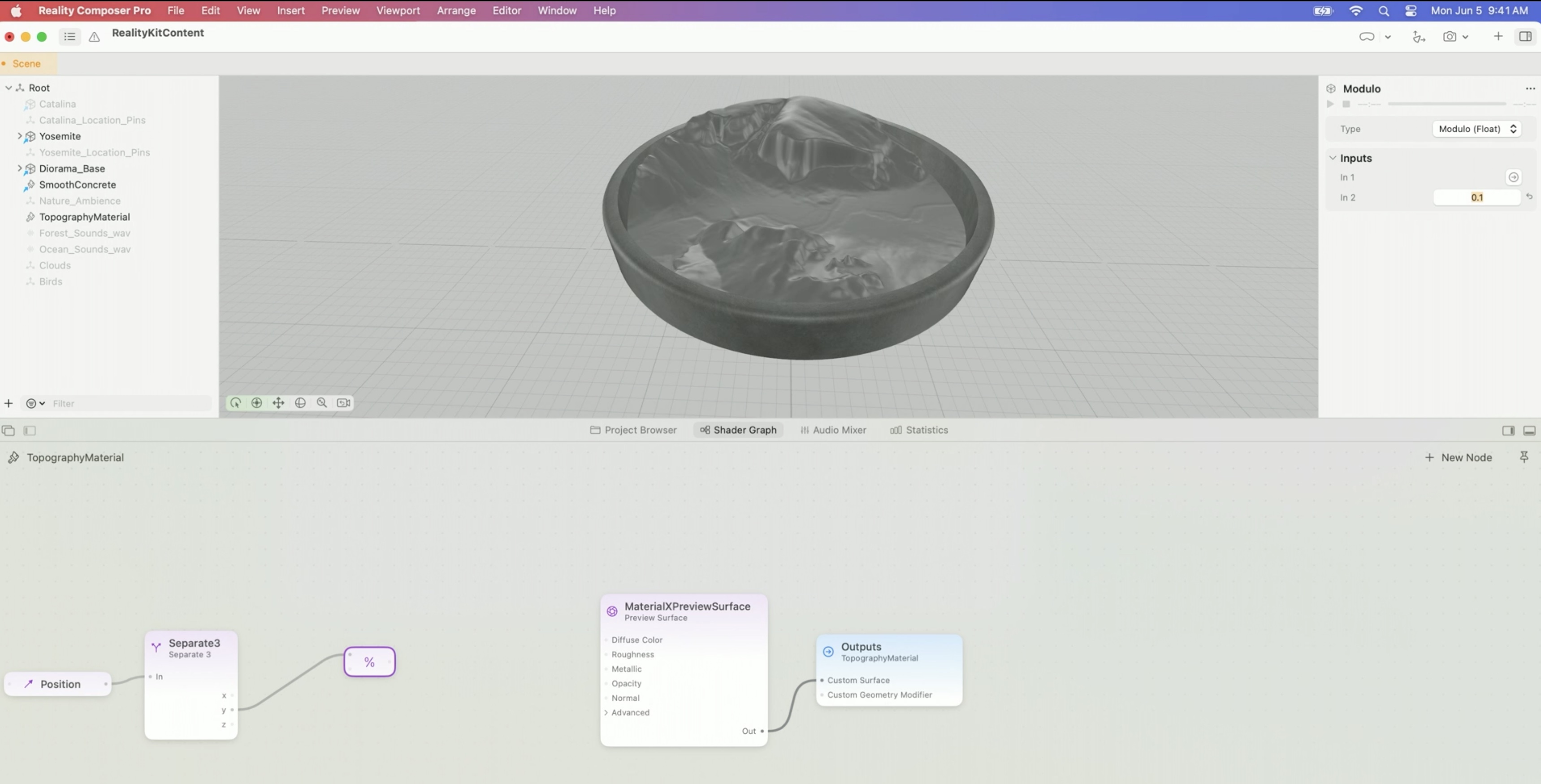
- Let’s add the modulo node to our material in Reality Composer Pro. Instead of double-clicking to add a node and then connecting it, we can drag a new connection to an empty space to create a node that’s already connected in one step. In the New Node picker, type “modulo” and click to insert a Modulo node. Modulo has two inputs. The first is the dividend and the second is the divisor. You can conveniently set constant values on inputs in the inspector instead of connecting nodes. In the inspector, change the second argument to 0.1. This is the divisor and sets the width of our height ranges.
- We have just one more step to go before we can see our output. We’ll use an ifgreater node to determine where our repeating values fall in narrow height bands on our terrain. The ifgreater node will return a value representing one of the two band colors you see on screen, depending on the result of a comparison. When the height is greater than our shader topographical line width, we’ll choose a background color. And where the height falls within our desired line width, we’ll choose our topography line color.
- ![] (https://www.wwdcnotes.com/images/notes/wwdc23/10202/yosemiteModel11.jpg)
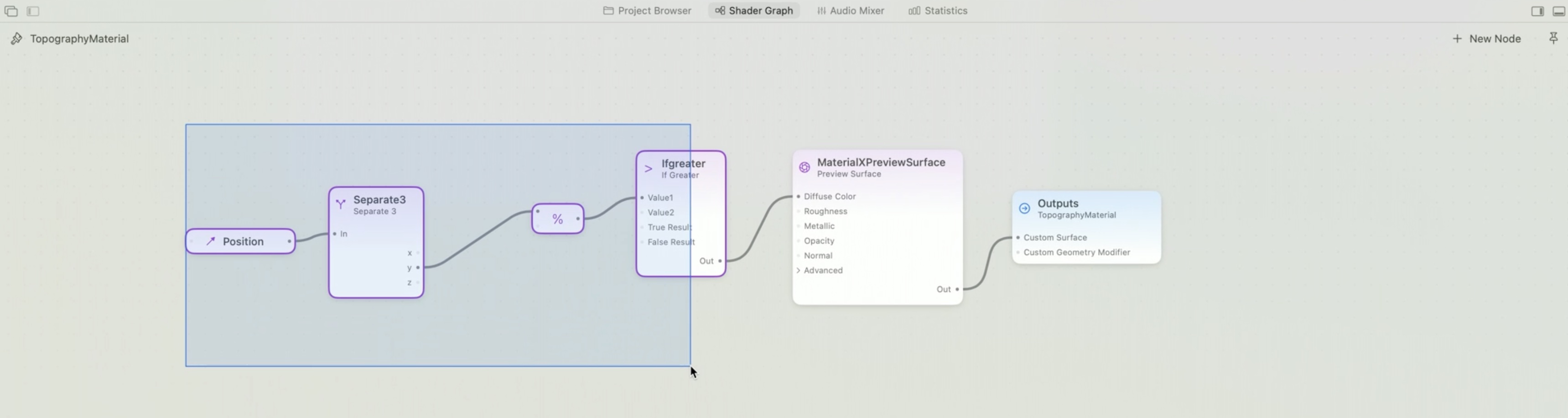
- Let’s add the ifgreater node to our material and see the results. We want to compare the result of the modulo node to a value we choose for our topographical line width. So I’ll add an ifgreater node to do that comparison. Ifgreater compares its two inputs and returns one value when its first input is greater than its second input, and a different value when the first input is less than its second input. This ifgreater node is set to output floating point values, but we want to choose between two colors, one for our terrain and one for our topographical lines. In the inspector, under Type, change this node to output RGB. Next, let’s pick our two colors.
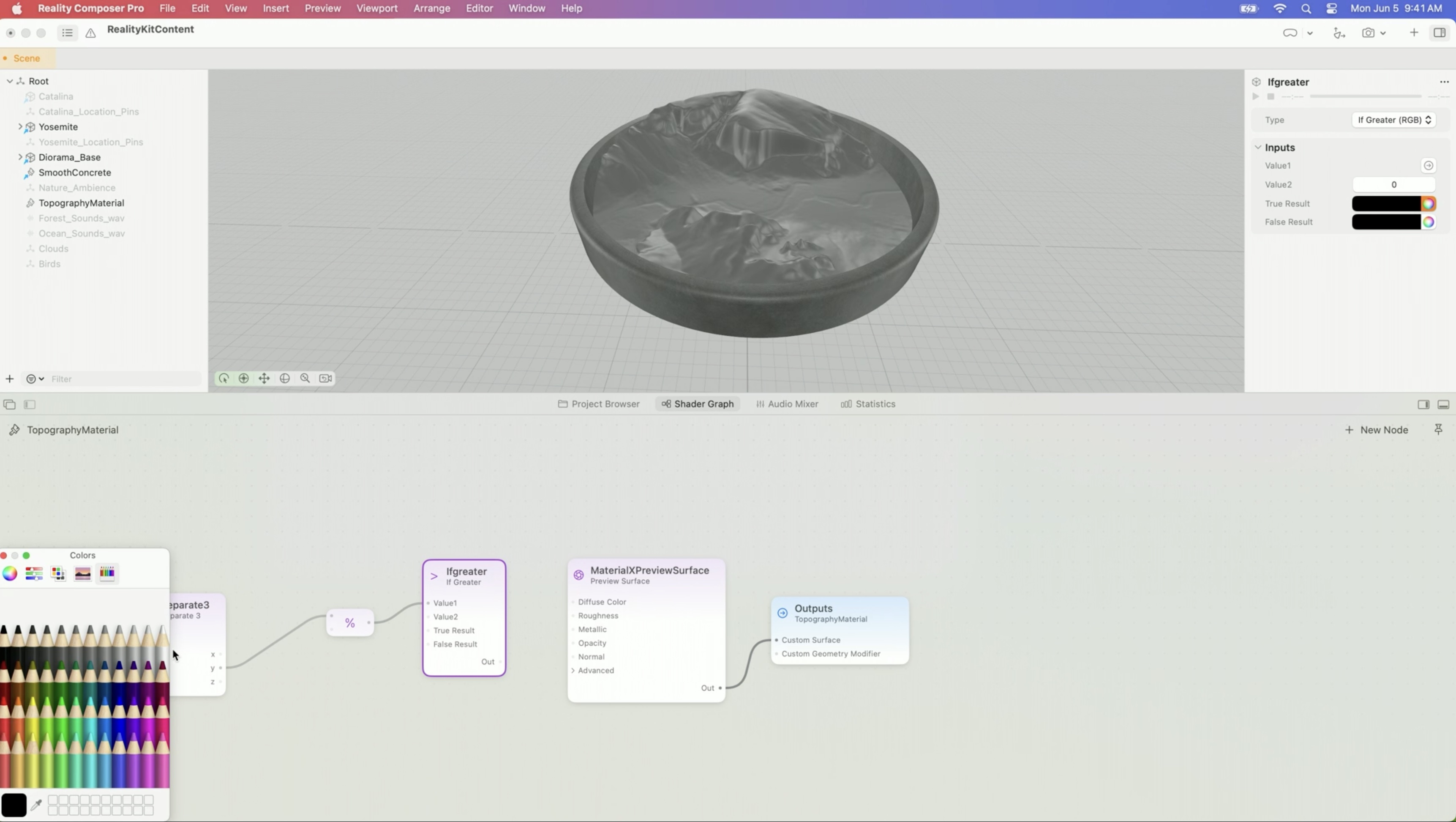
-
In the inspector, I’ll click on the color picker next to True Result and set our terrain color. Let’s use white. Let’s leave the False Result, which is our topographical line color, set to black.
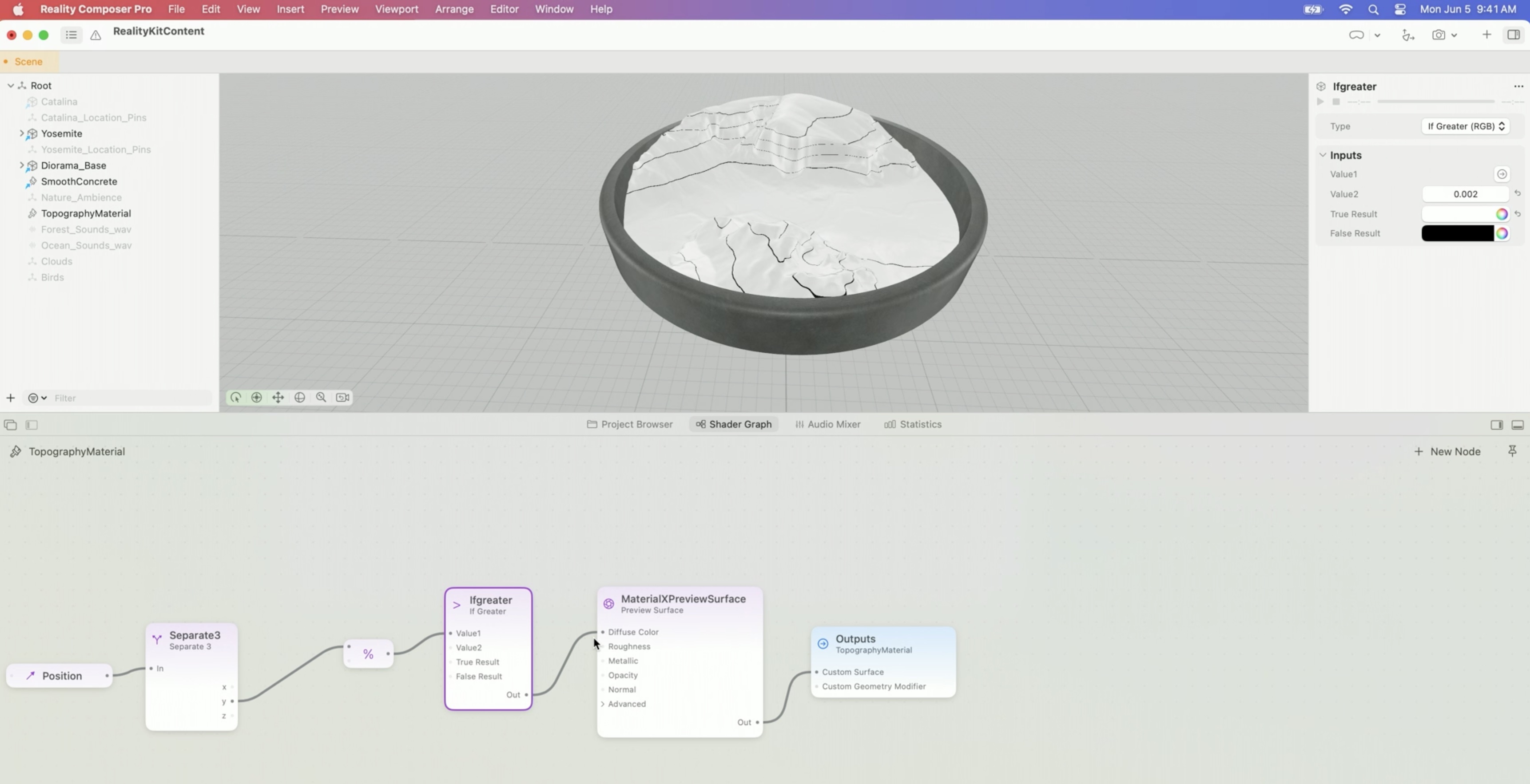
- This will give us a lot of contrast with our white terrain. I tried a bunch of values and arrived at 0.002 as a good value for line width, so in the inspector, I’ll set my comparison value to 0.002. I’ll connect the ifgreater node’s output to our surface’s Diffuse Color input. Awesome, now our material is setting the color at every point on our terrain and we’ve made a topographical lines material.
- Regarding this tutorial there are a few questions
- How do we obtain the size of the Yosemite.usd file to suggest that 0.1 represents 1000ft?
- No idea yet, will check out Explore the USD ecosystem
- Is a line width of 0.002 represent 2 ft?
- Answer, yes probably.
- Why does ifgreater work? I mean shouldn’t it be greater or less than, because less than the number would result in true right?
- Answer, it is within the narrow band of 0.002 of the modolo number to create the lines
- How do we obtain the size of the Yosemite.usd file to suggest that 0.1 represents 1000ft?
Node graphs
- Node graphs help simplify complex materials and let you create your own nodes to reuse parts of graphs
-
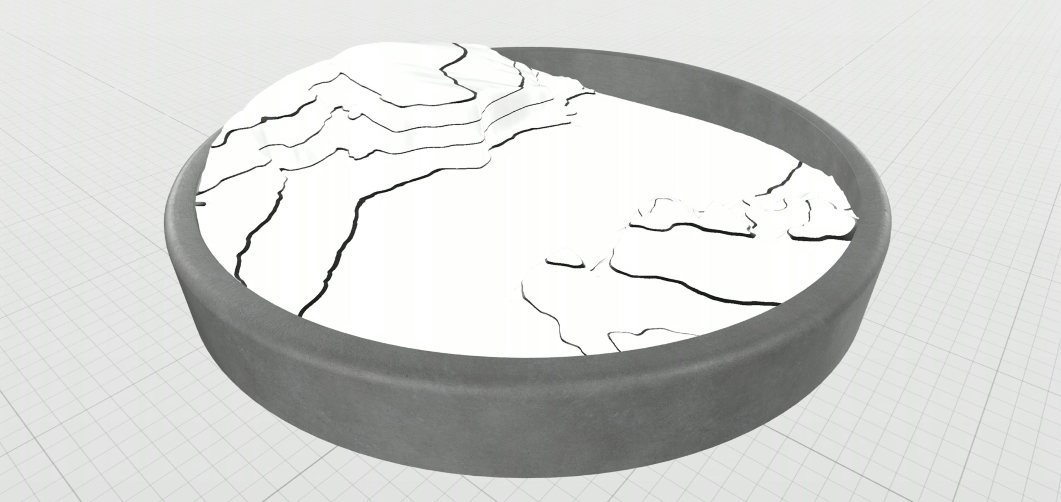
We’ll use node graphs to give a material a real topographical map look. Let’s add a second set of lines between the current lines of our material.
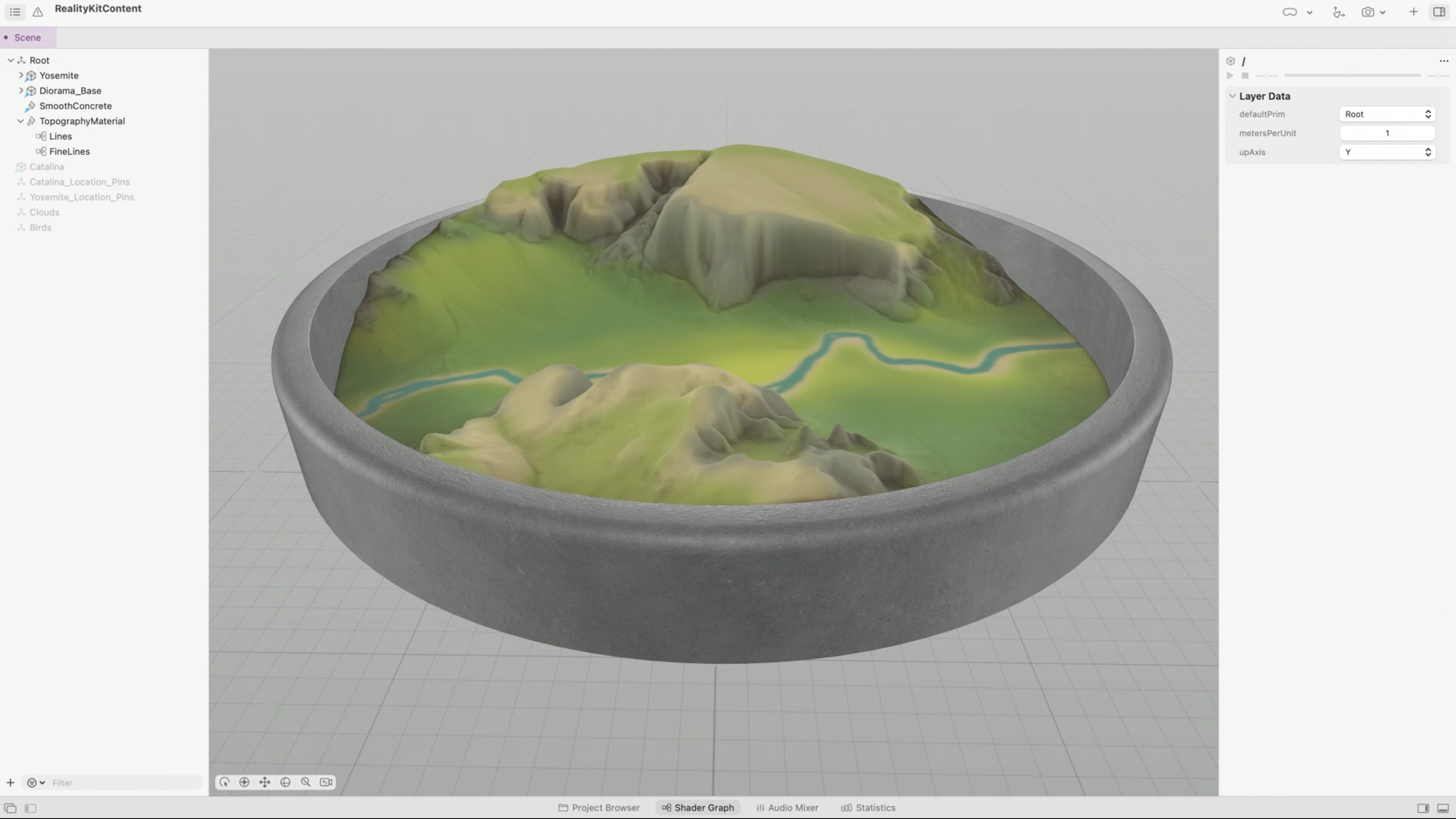
- Here’s what our material looks like so far.
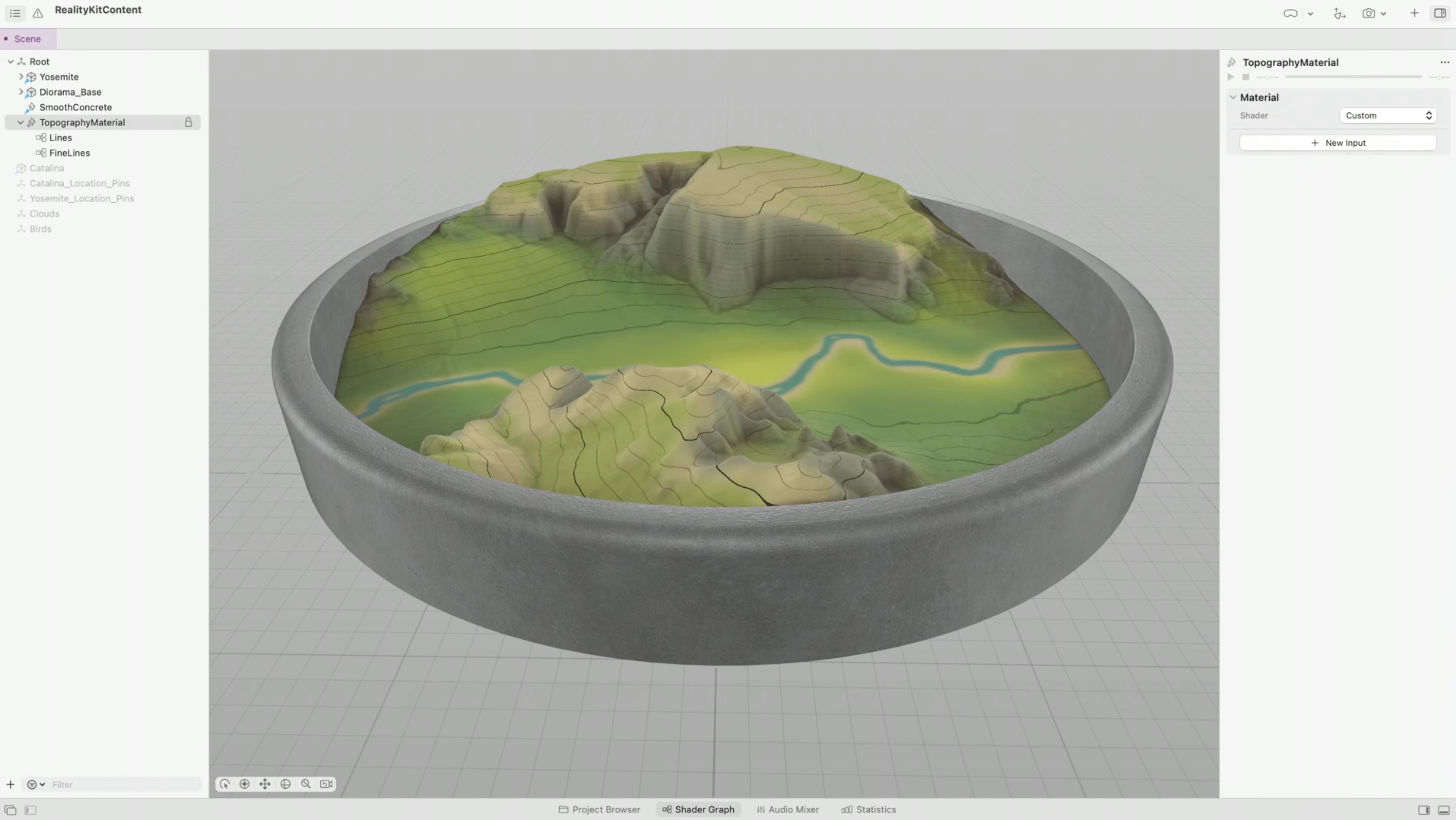
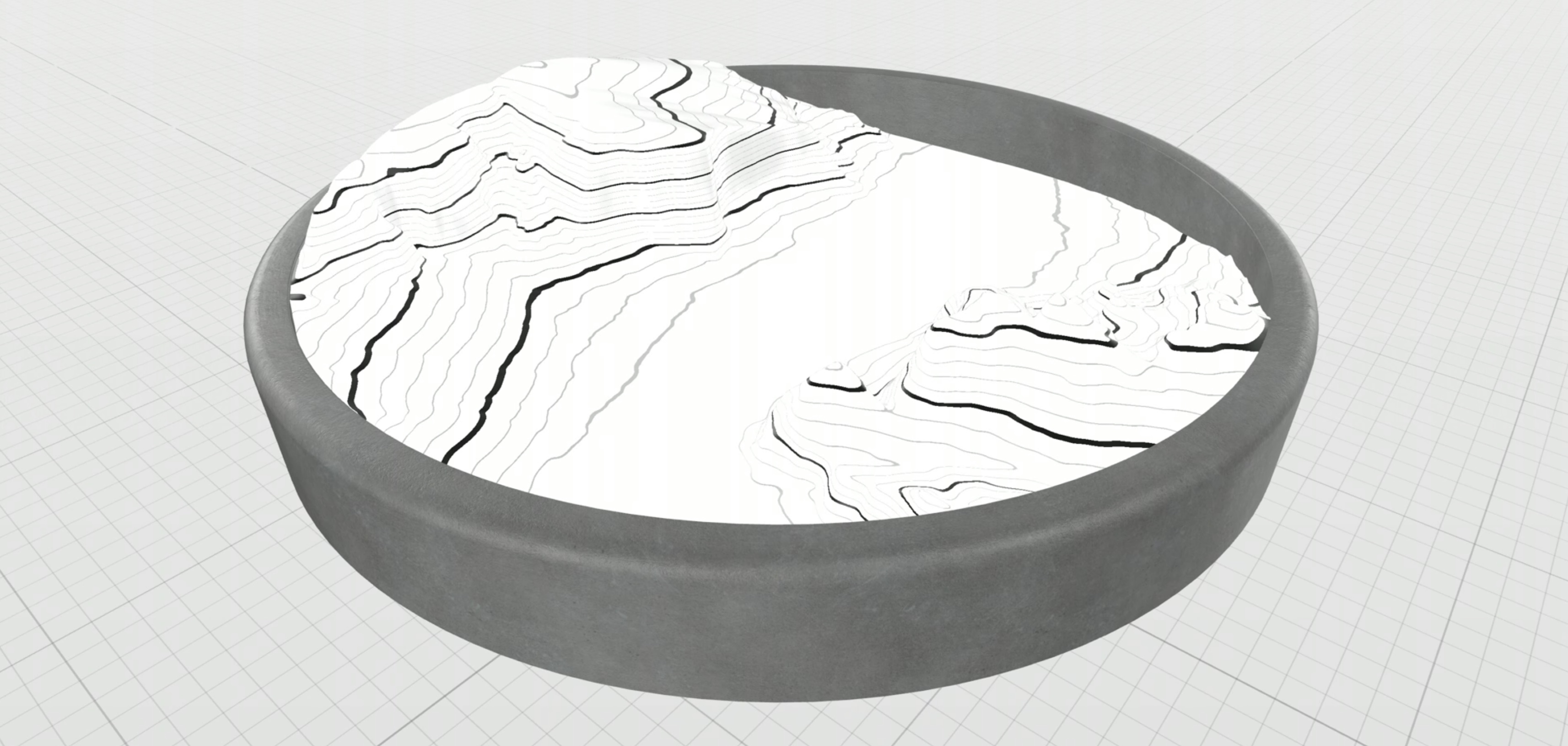
- And here’s what it will look like when we add our subdivisions.
- We’ll start with the four nodes in our material that draw our topographical lines.
- Then we’ll compose a node graph from them. This will combine our four nodes into a single node. Finally, we’ll create an instance of our node graph to reuse its functionality. One node graph will draw our original set of lines, and the instance of it will draw our second set of lines.

- Let’s go back into Reality Composer Pro and build it. Here is our topographical lines shader again. Drag to select these four nodes that compute the colors for our lines and where to draw them.
- After selecting them, right-click and choose Compose Node Graph. Now the nodes appear as a single node that I can use inside other graphs. Let’s assign a descriptive name to our new node. Let’s call it Lines. Multi-select any set of nodes and right-click > Compose Node Graph to make reusable node components 11:21.
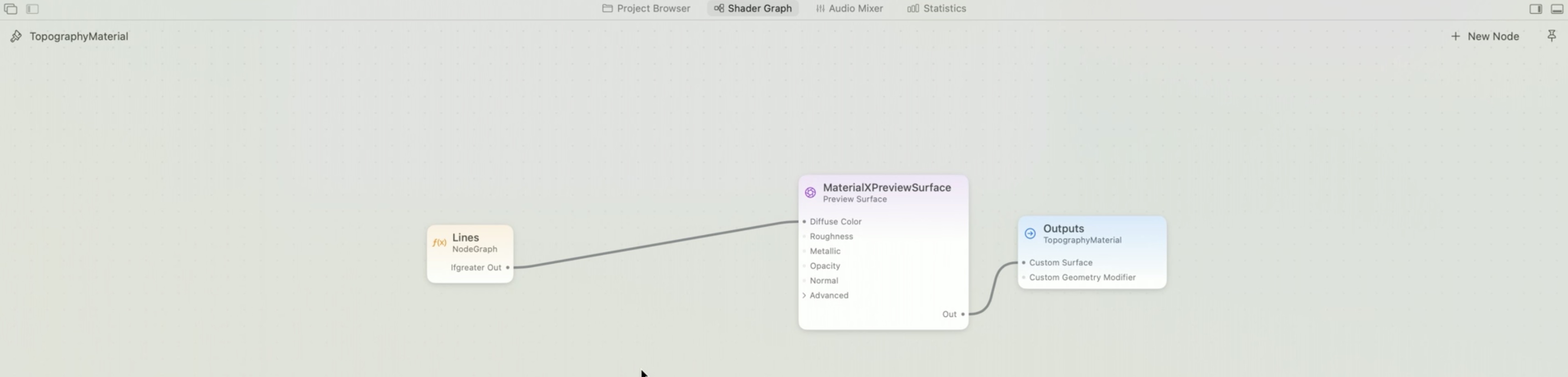
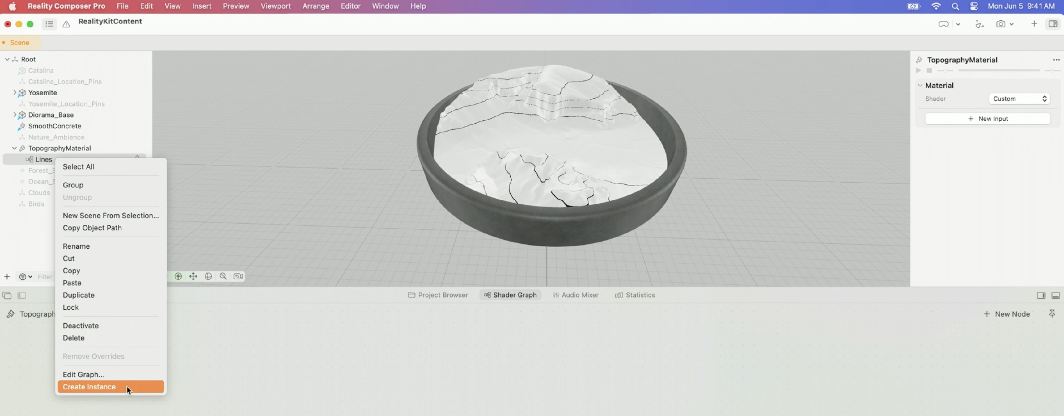
- We’ll create a copy of this node graph to draw our second set of lines. For this, I’ll create an instance using the Create Instance command in the hierarchy. In the project hierarchy, right-click > Create Instance to create an instance of your node graph 11:35.
- Instances are live copies that adopt any changes made to the original node graph. We’ll return to our material by selecting it. Let’s call our new instance SecondaryLines.
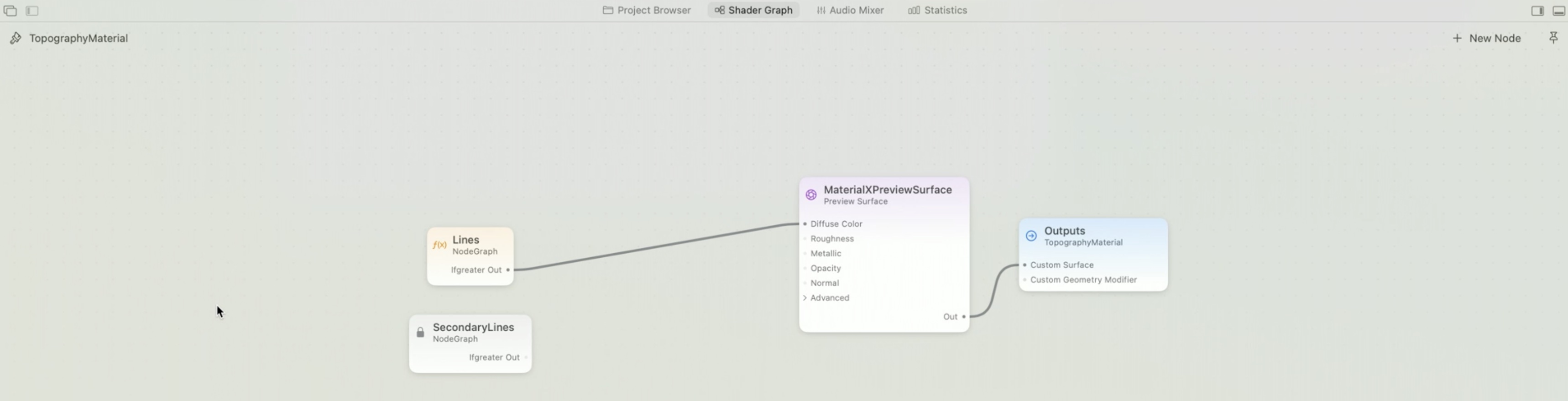
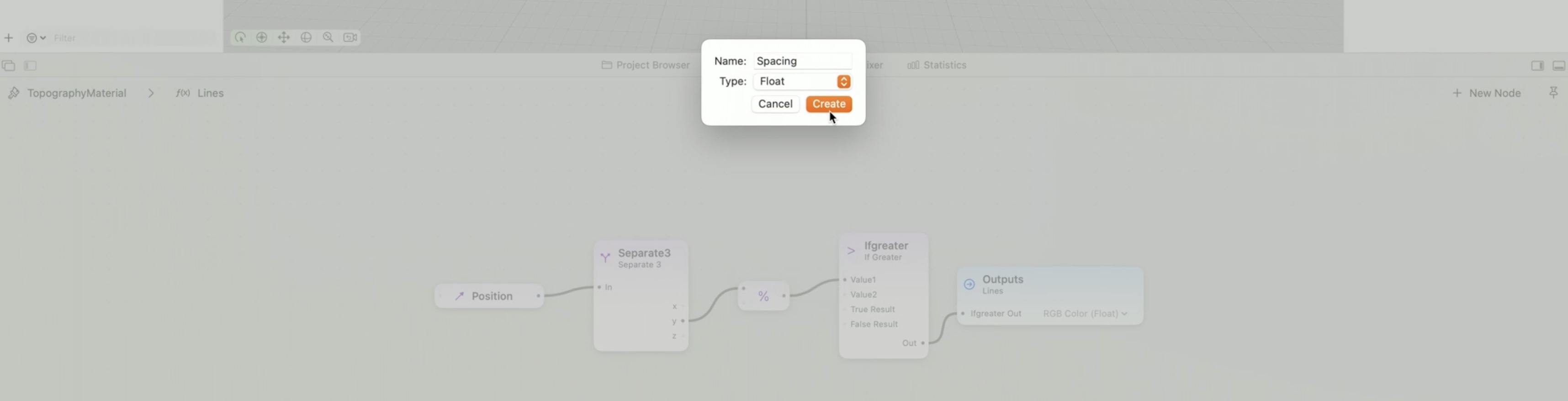
- We want our node graph and its instance to draw lines with different spacings and colors, so we’ll add two inputs, called Spacing and Color, to our original node graph to control these properties. Let’s edit our original node graph by double-clicking it. You add inputs and outputs to your node graph in the inspector. First let’s add an input called Spacing and set its type to Float.
- We’ll also add an input called Color to control our topography line color. Set the type of the input to Color3.
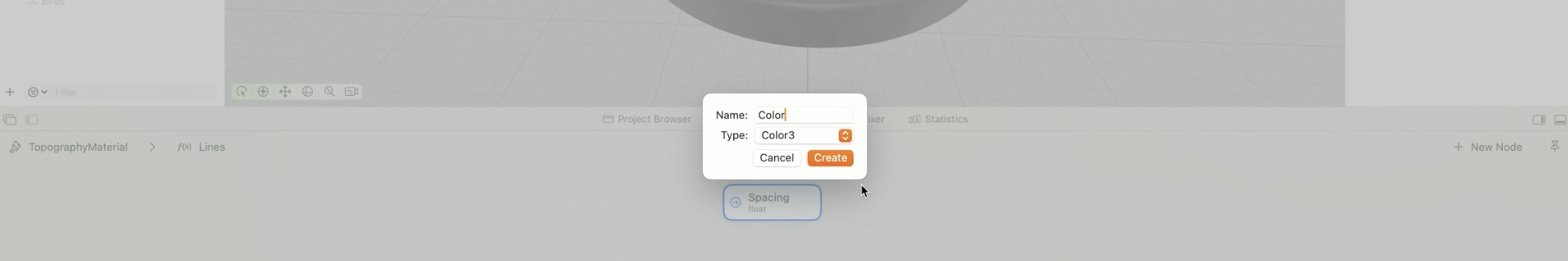
- I’ll connect these to the right places in our graph. Add inputs and outputs to your node graph in the inspector 12:10.
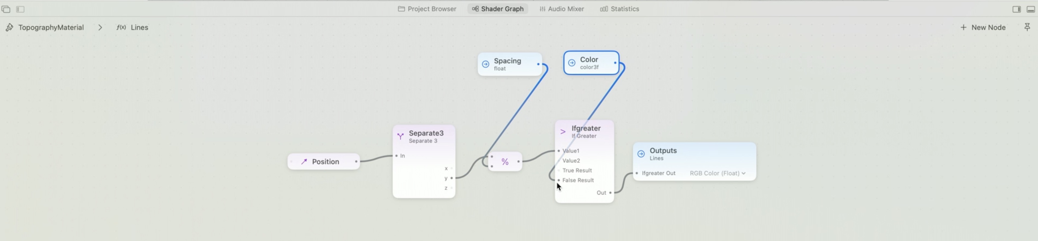
- Let’s go back to our material by selecting it in the project hierarchy. Notice that our node graph now has the two inputs we created, and that our instance inherited these two new inputs. On the original Lines node graph, set spacing to the values we chose before. And let’s choose a smaller spacing and a lighter color for our instance node graph. The last step is to combine the outputs from our original and instance node graphs. I’ve conveniently chosen grayscale colors for both node graphs, so we can combine their colors using a multiply node.
- NOTE: Instances of node graphs are live copies that adopt any changes made to the original node graph. They inherit inputs and outputs added to the original node graph it points to.
Geometry modifiers
- These are a feature of custom materials you can use to modify your models in real time. Walk-through tutorial on applying heightmaps to generate geometry, and animating between those heightmaps. Starts at 13:46.
- We’ll replace our static terrain model and recreate it using geometry modifiers and height data. Then we’ll extend our geometry modifier to dynamically animate between two different terrains: Yosemite Valley and Catalina Island, California. When we’re done, we’ll have a dynamic terrain material that can animate between our two different locations. Let’s see how this is done. All the shaders we’ve looked at so far are surface shaders. These are shaders that set the physically based, or PBR, attributes for each pixel of our model as it’s rendered. Geometry modifiers are similar to surface shaders, but operate on the geometry of your objects instead. In fact, you build them right in the same editor in Reality Composer Pro.
- Reminder Surface shaders operate on the PBR attributes while Geometry modifiers operate on the geometry of objects.
- Let me give you an overview of the geometry modifier we’re going to build that will create a terrain of Yosemite Valley using its height map data. We’ll start with a flat disk model, which contains some plain geometry. This will be our base surface. Next we’ll use our terrain height data, which is 2D data about the height at each location of our model, and use a geometry modifier to raise the terrain by the correct amount. This will result in the terrain we want. Once I’ve shown the basic version, I’ll demonstrate a version that takes two sets of terrain heights and uses those to animate between our two locations of interest, Yosemite Valley and Catalina Island.
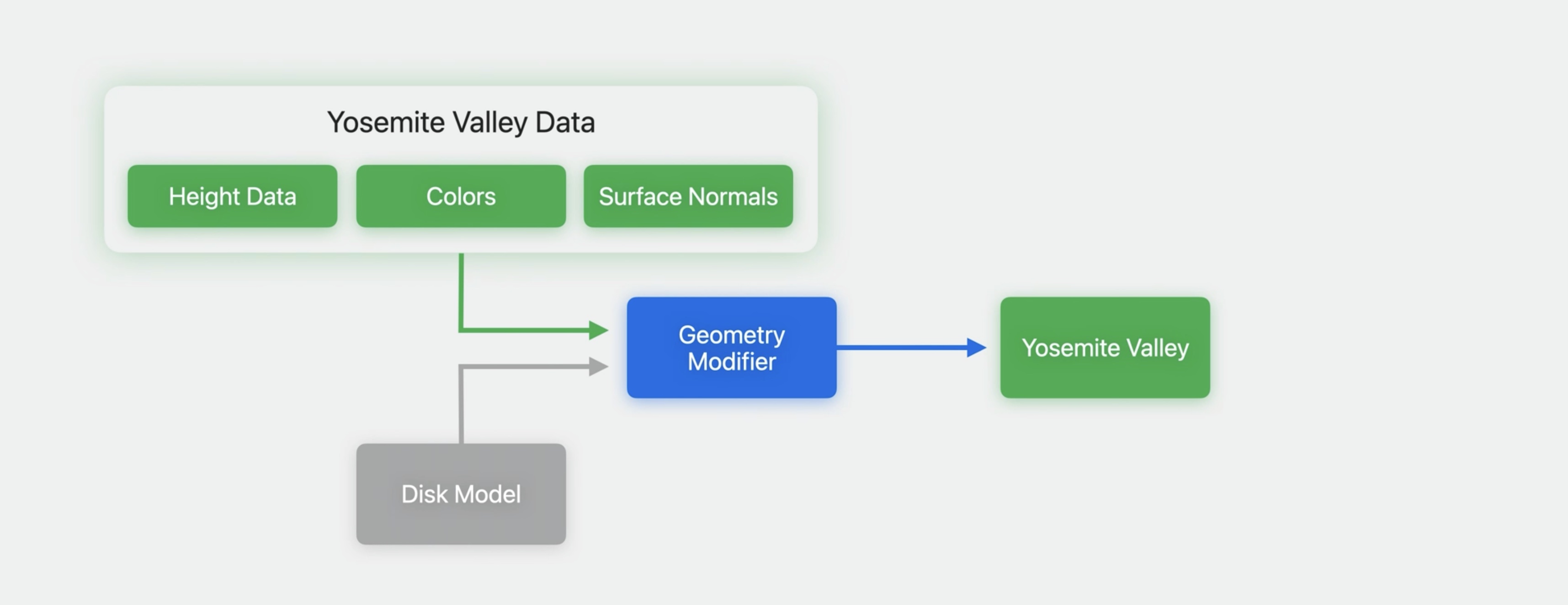
- Here’s another view. We’ll start with a flat model, and our geometry modifier will move its vertices vertically using data from a 2D height map like this.

- The first thing we’ll do is use the Deactivate command to hide the prebuilt Yosemite Valley model.
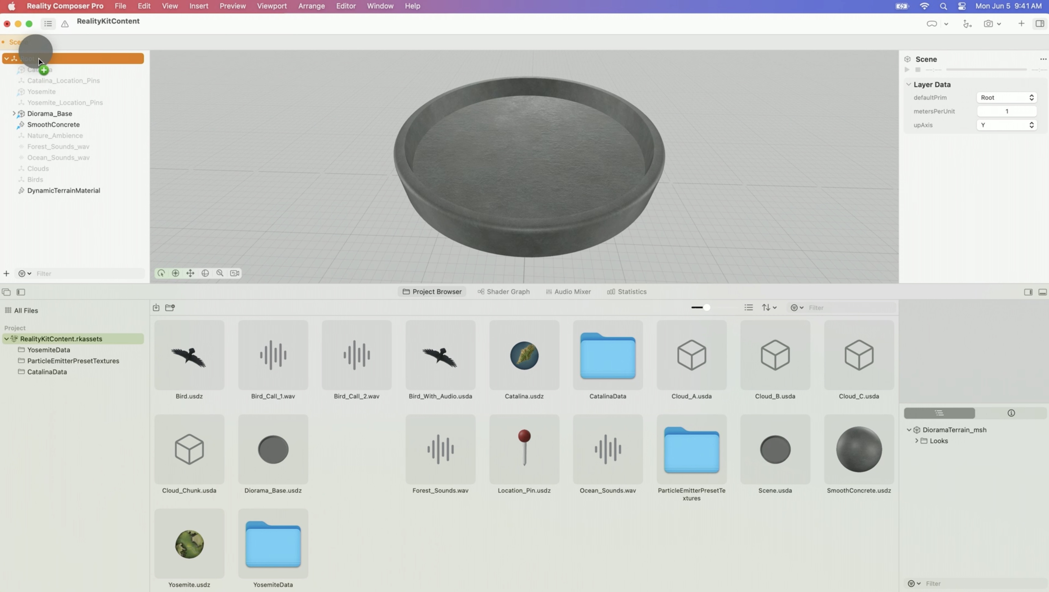
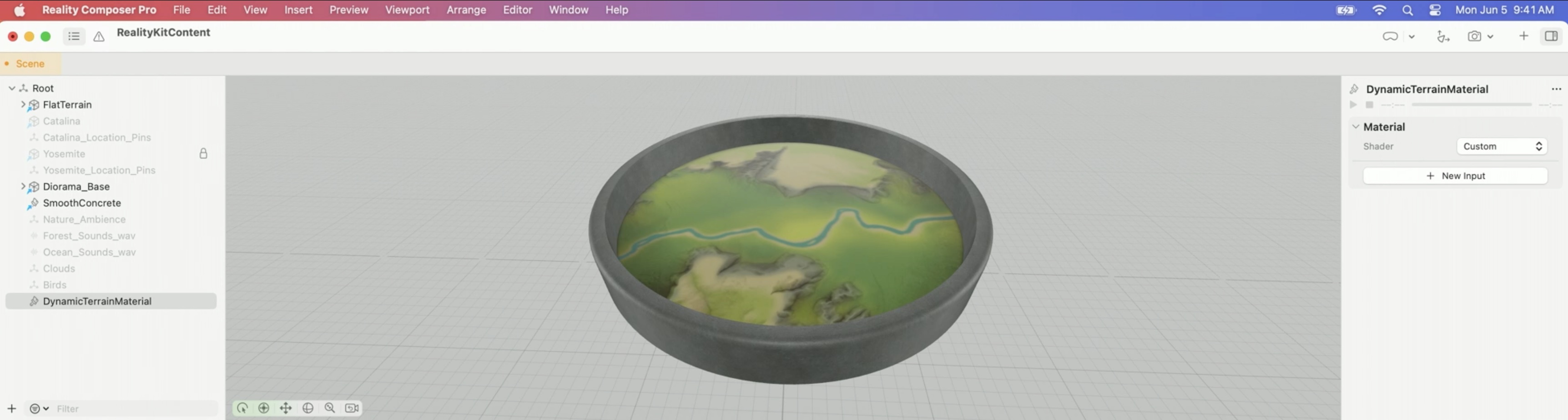
- We’ll generate the same Yosemite Valley model, but this time using our geometry modifier. I’ll start with a flat disk model in my Project Browser. I can bring it in by dragging it into the Root entity in the project hierarchy.
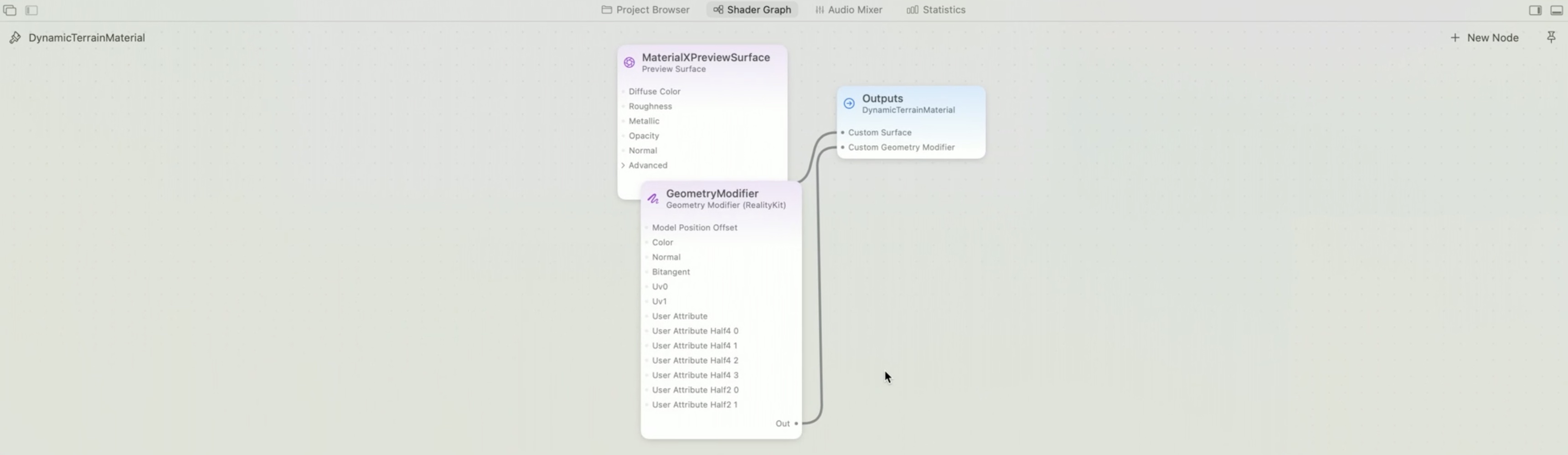
- I’ve gone ahead and created a new material named DynamicTerrainMaterial and assigned it to the disk. Let’s get to work on our geometry modifier. In the Shader Graph editor, we’ll need a geometry modifier surface. We’ll add this to our material alongside our PBR surface. I’ll drag a connection from the Custom Geometry Modifier input of our output node and choose Geometry Modifier from the New Node UI.
- Let’s first apply our Yosemite Valley image to our surface. To read image data, we’ll use an image node.
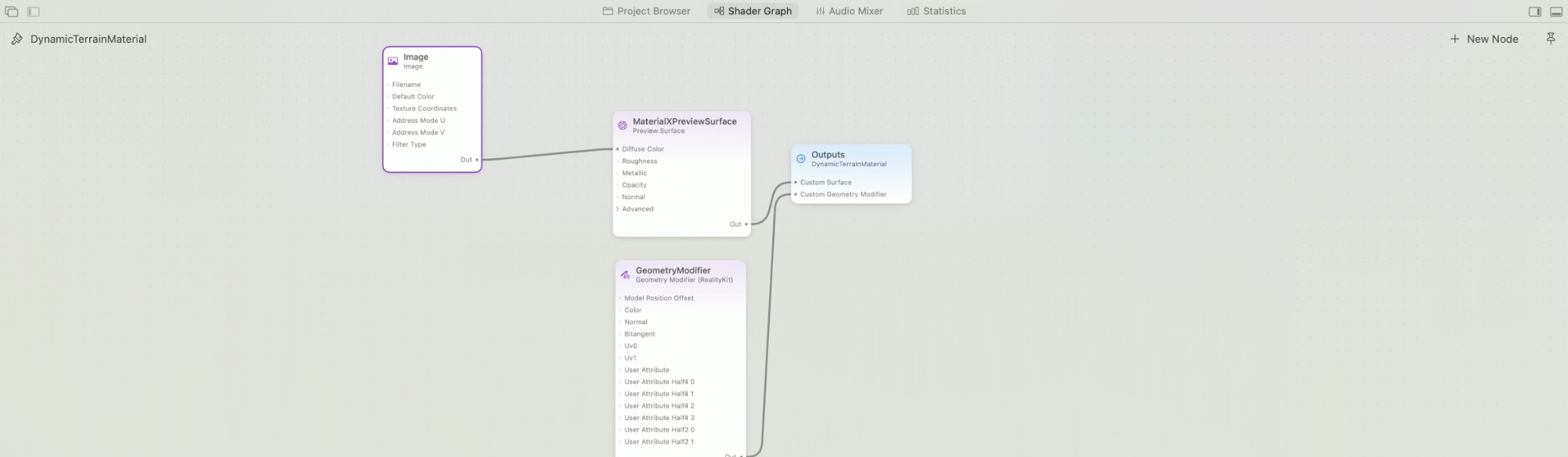
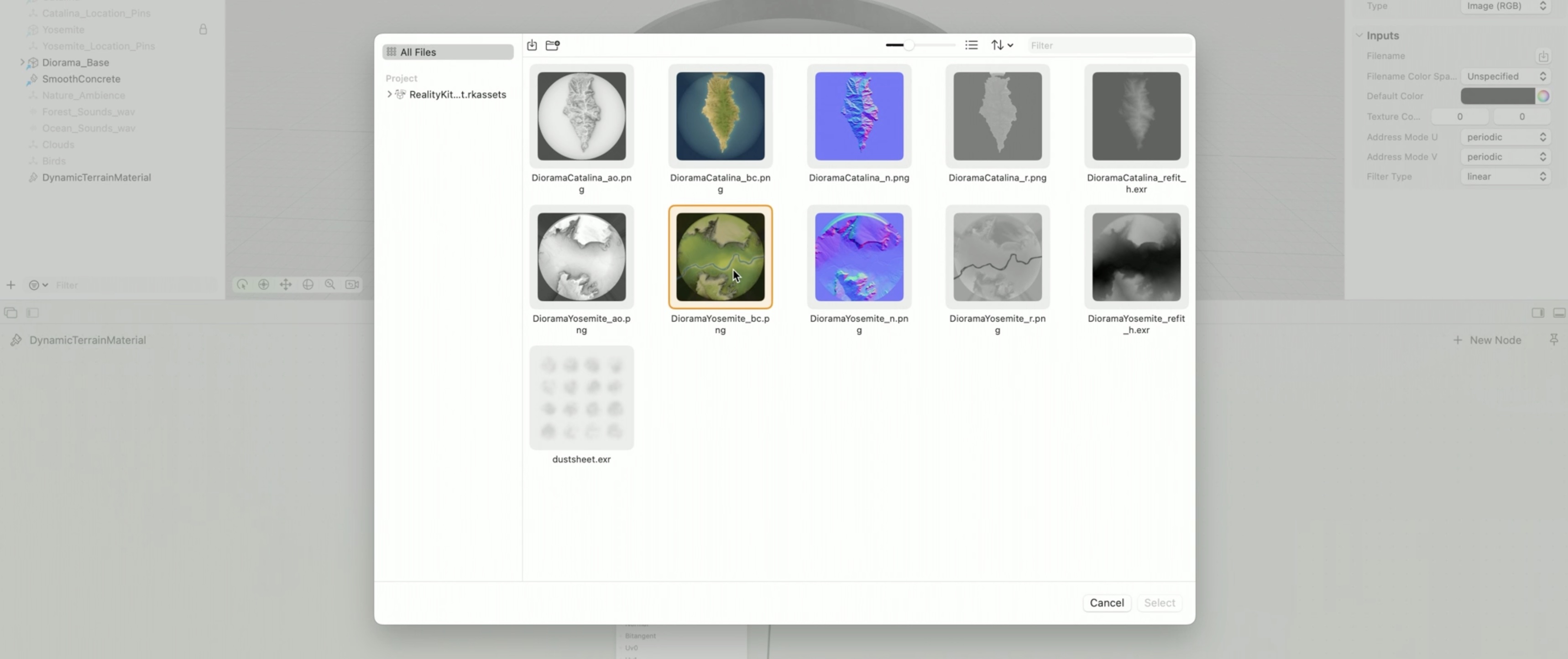
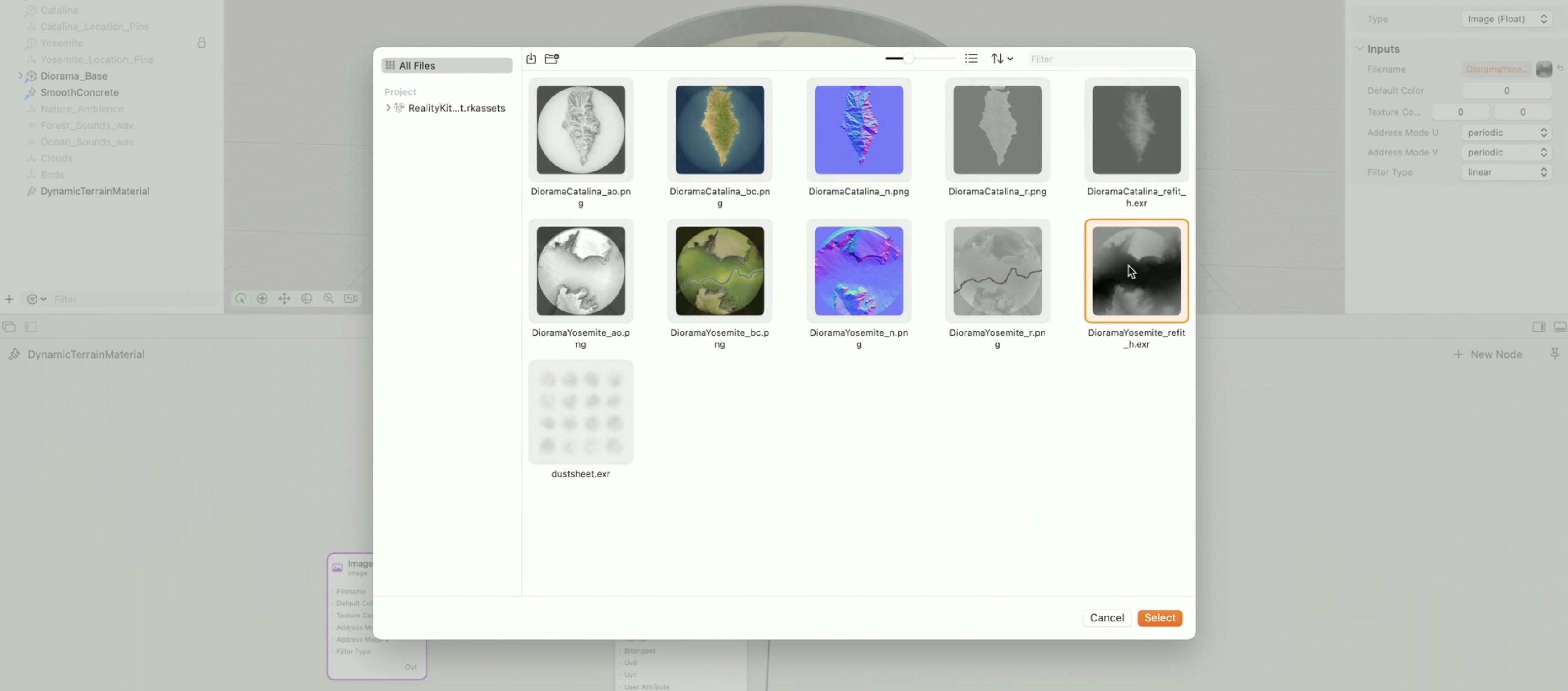
- In the inspector, let’s assign our Yosemite Valley image to the image node’s Filename input.
- Things look a bit funny since the terrain is flat, but we’re going to fix that now.
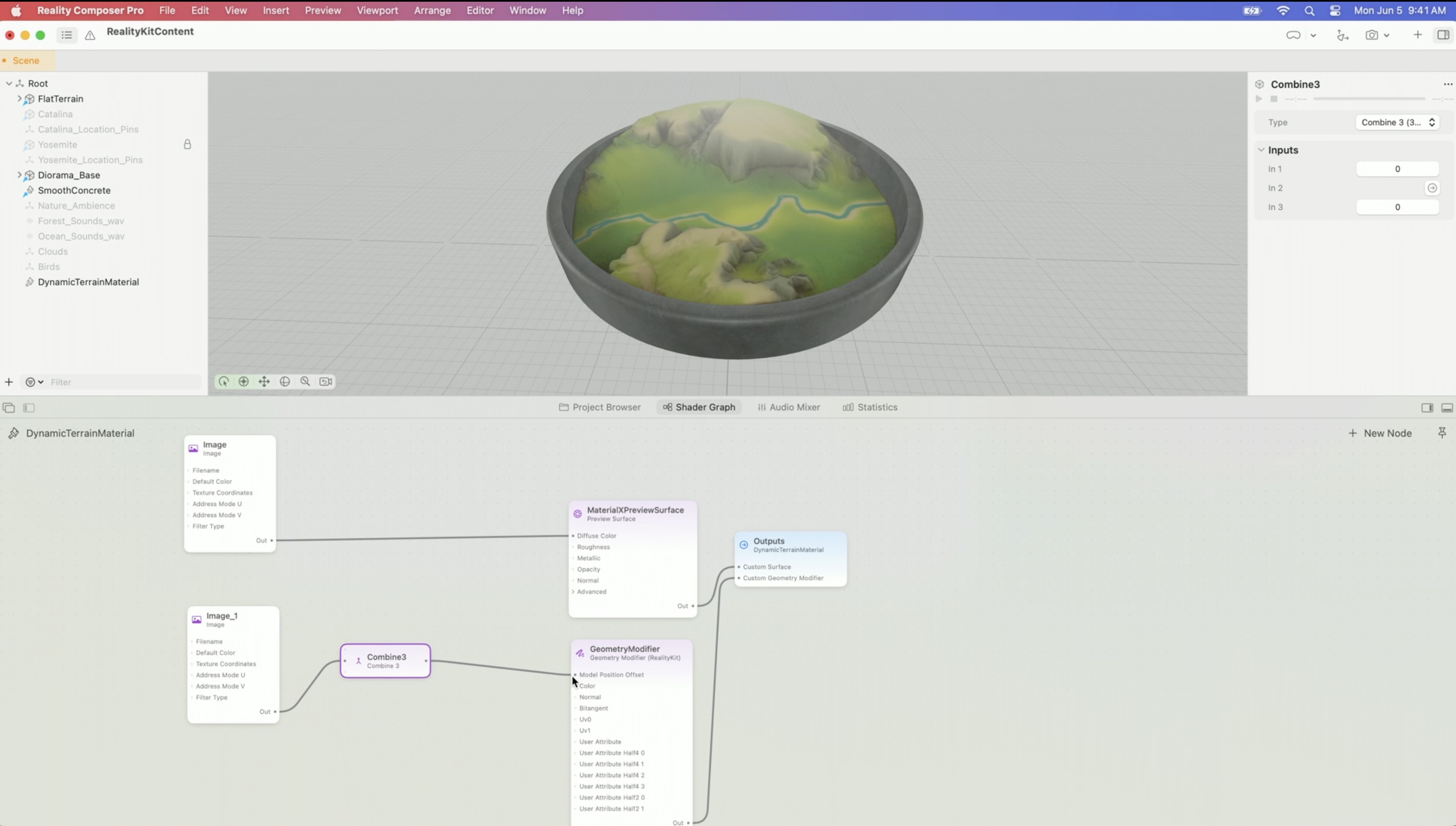
- We’ll need the height data for our valley. It’s in an image file which contains height values instead of color data. Since this data is in an image, we’ll read it by adding another image node. Now assign our Yosemite Valley EXR image containing our height data to this new image node’s Filename input.
- Geometry modifiers can move the vertices of our model in any direction, but we’re only interested in moving them vertically, so let’s insert a Combine 3 node to create a 3D vector with only the Y component set. Now connect this to the GeometryModifier surface’s Model Position Offset input, and boom, our flat model has been transformed into Yosemite Valley.
- There’s one more step we need to take. When we move our vertices, we’ll also need to set the surface normal vectors of our model to match our new terrain shape. There are ways to compute these from the height data, but today we’re going to use an image that contains precomputed normals for this geometry. Let’s create another image node to read the normals.
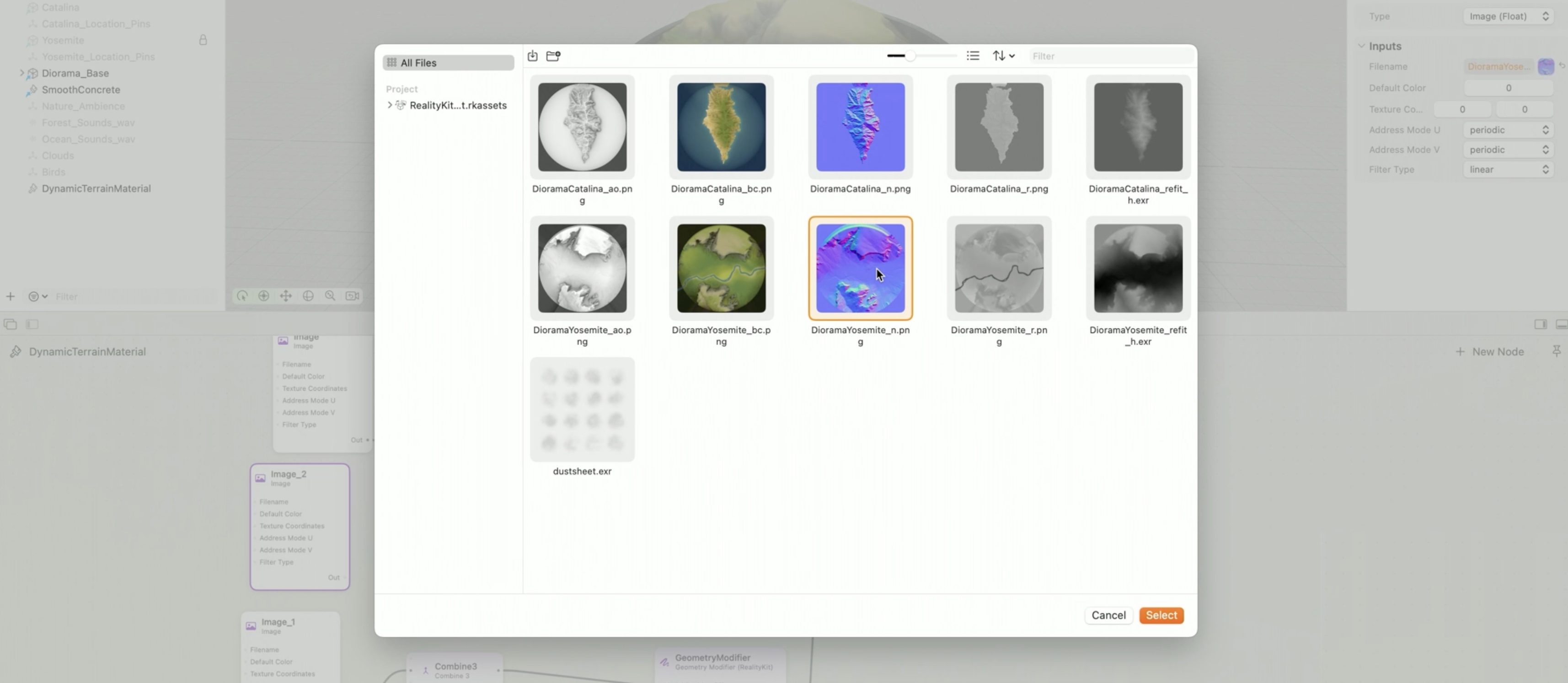
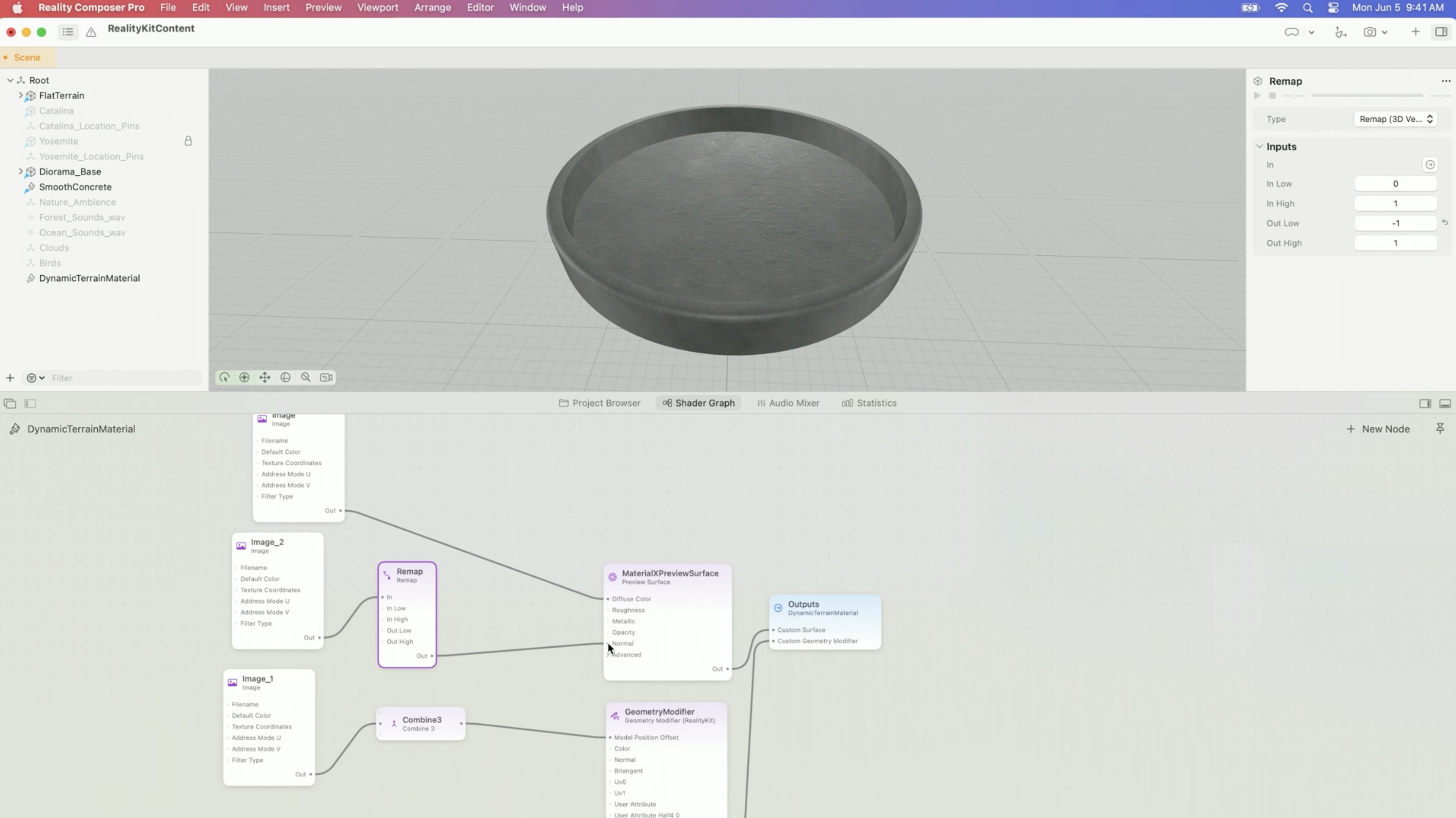
- Since these are precomputed, we’ll connect them directly to our surface shader’s normal input for better accuracy. Our surface expects normals to have values between -1 and 1, but the normals in our image are between 0 and 1. I’ve remapped the values from the image using a remap node.
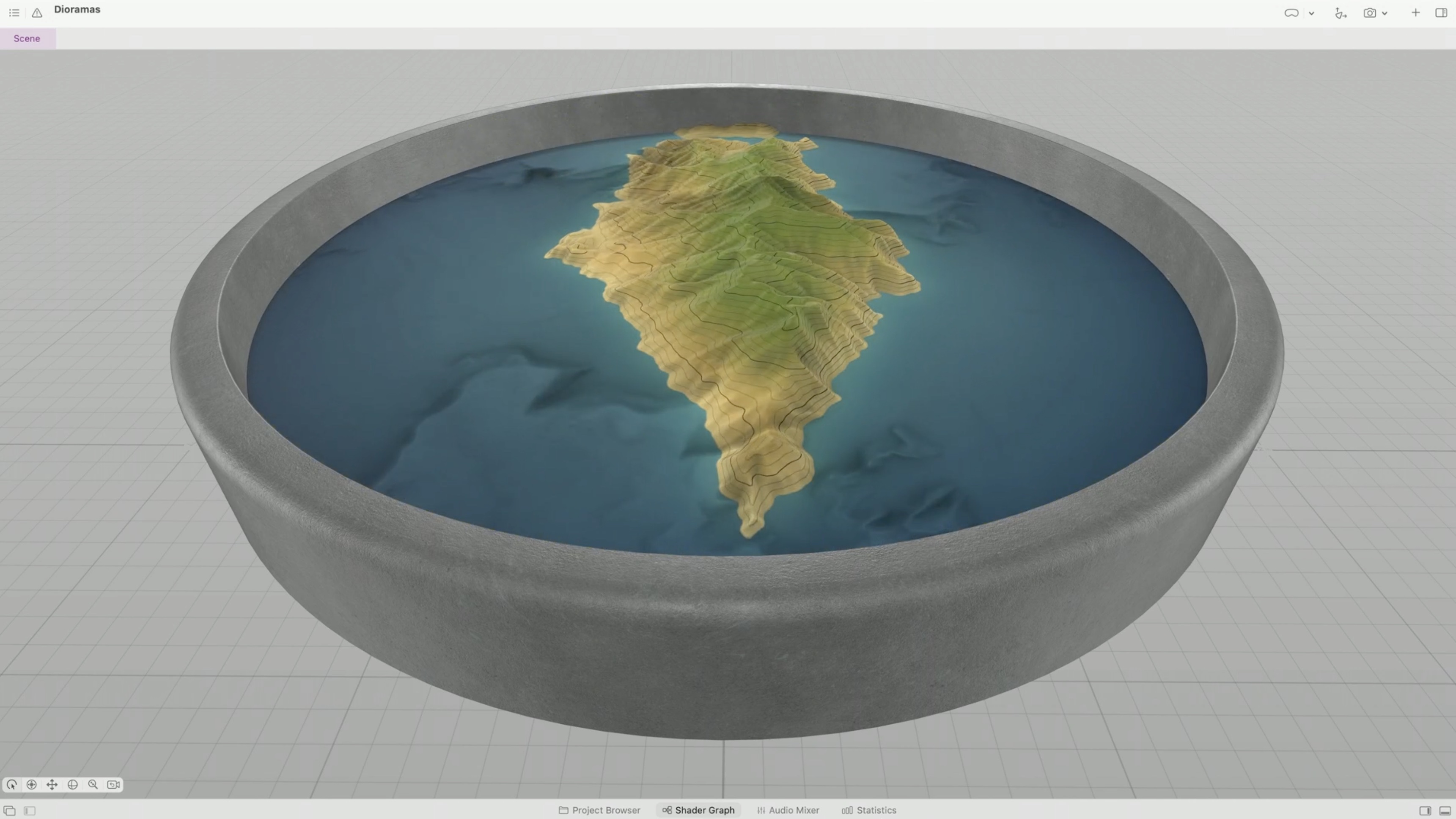
- Now we’ve created the terrain from a flat geometry using height data. Next, let’s make our diorama dynamic and add the ability to morph from one terrain to another. In this case, we’ll add an animated transition to change Yosemite Valley to Catalina Island. To achieve this, we’ll first add another set of image nodes to our existing geometry shader. The nodes contain the heights, colors, and normals for our Catalina Island terrain. Then we’ll add mix nodes to blend between these two sets of heights, normals, and colors. Finally, we’ll connect a value to our mix nodes to control blending between our two sets of data.

- Let’s build this in Reality Composer Pro now. OK, here’s our material so far.
- 
- Next I’ll add some mix nodes to blend between our two colors, heights, and normals.
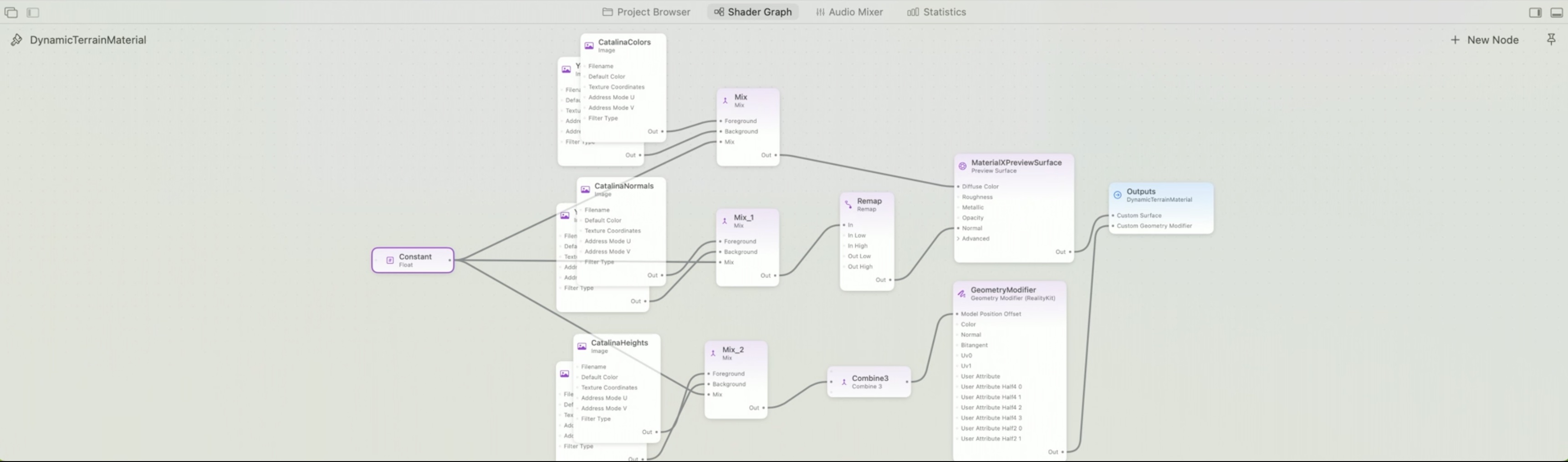
- Finally let’s connect a 0 to 1 constant to our mix nodes, which will control which terrain is shown. You’ll notice when I set my mixing constant to 1, the terrain shows Catalina Island. When I set the mixing constant to 0, we see Yosemite Valley.
- Now that we have a material that can transition between our two different terrains, let’s make this transition progress value changeable from our Swift code. We’ll use the Promote command to convert our progress value into an input on our material.
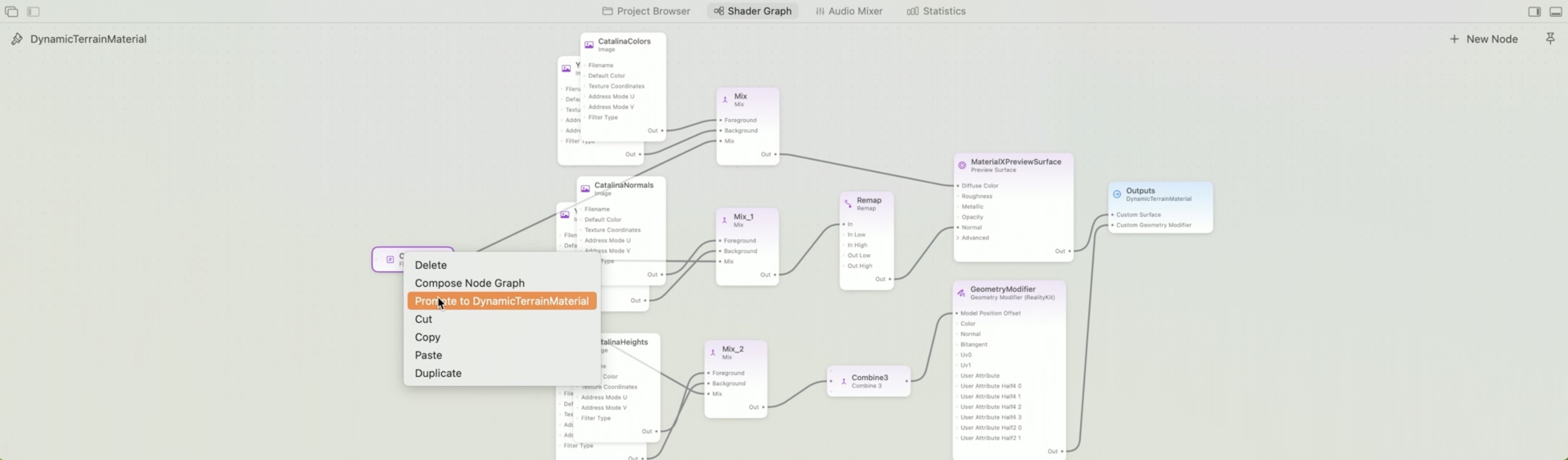
- Inputs on materials become properties of your material that can be accessed from your Swift code. Now our material is ready to be used in our Dioramas Swift app. Here’s the final version, which combines our topography lines and our dynamic terrain. This version has some additional refinements, like anti-aliased topography lines and ambient occlusion maps, all added using Shader Graph.